Gradient computation example

Minimal example visualizing the gradient of a scalar function on a mesh

import numpy as np
from mayavi import mlab
import trimesh

from bfieldtools.viz import plot_data_on_vertices
from bfieldtools.mesh_calculus import gradient
import pkg_resources

# Load simple plane mesh that is centered on the origin
file_obj = file_obj = pkg_resources.resource_filename(
    "bfieldtools", "example_meshes/10x10_plane.obj"
)
planemesh = trimesh.load(file_obj, process=False)

# Generate a simple scalar function
r = np.linalg.norm(planemesh.vertices, axis=1)
vals = np.exp(-0.5 * (r / r.max()))

# triangle centers for plotting
tri_centers = planemesh.vertices[planemesh.faces].mean(axis=1).T
tri_centers[1] += 0.1

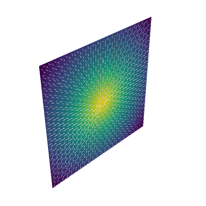
Calculate the gradient (e.g., flow from potential)

g = gradient(vals, planemesh, rotated=False)

# Plot function and its gradient as arrows

scene = mlab.figure(None, bgcolor=(1, 1, 1), fgcolor=(0.5, 0.5, 0.5), size=(800, 800))

plot_data_on_vertices(planemesh, vals, ncolors=15, figure=scene)
vecs = mlab.quiver3d(*tri_centers, *g, color=(1, 1, 1), mode="arrow", scale_factor=5)
vecs.glyph.glyph_source.glyph_position = "center"

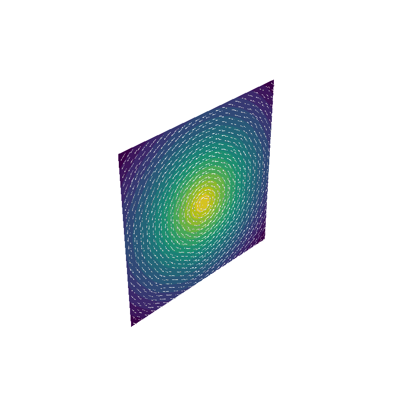
The same but rotated (e.g. current density from a stream function)

g = gradient(vals, planemesh, rotated=True)

# Plot function and its gradient as arrows
scene = mlab.figure(None, bgcolor=(1, 1, 1), fgcolor=(0.5, 0.5, 0.5), size=(800, 800))

plot_data_on_vertices(planemesh, vals, ncolors=15, figure=scene)
vecs = mlab.quiver3d(*tri_centers, *g, color=(1, 1, 1), mode="arrow", scale_factor=5)
vecs.glyph.glyph_source.glyph_position = "center"

Estimated memory usage: 114 MB