Note
Go to the end to download the full example code.
Thermal noise of a star-shaped conductor
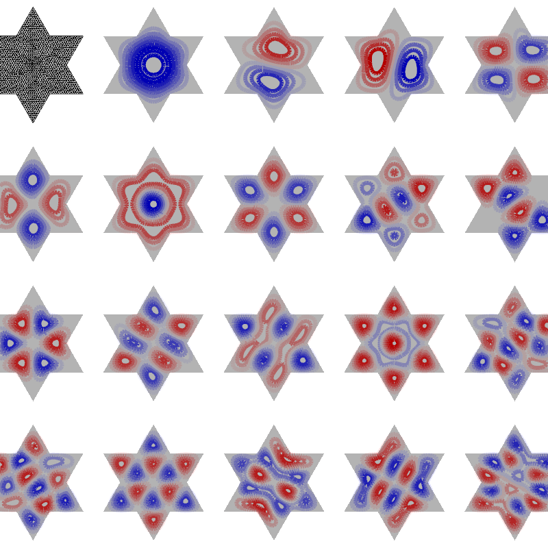
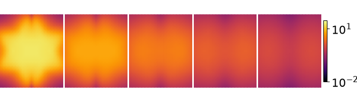
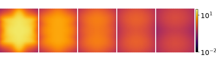
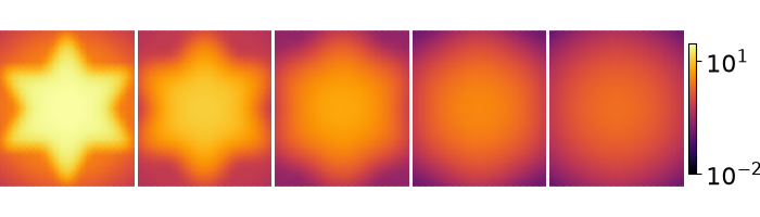
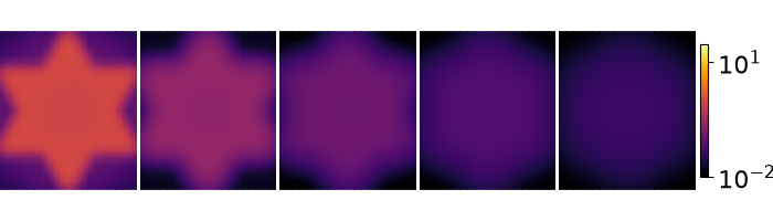
Visualize current modes and compute thermal magnetic noise for a star-shaped conducting surface.
import pyvista as pv
from bfieldtools._example_plots import mesh_actor
from bfieldtools._example_plots import triangle_mesh

pv.set_plot_theme("document")

import numpy as np
import matplotlib.pyplot as plt
import trimesh
from bfieldtools.thermal_noise import (
    compute_current_modes,
    noise_covar,
    noise_covar_dir,
    noise_var,
    visualize_current_modes,
)
from bfieldtools.mesh_magnetics import magnetic_field_coupling

from bfieldtools import resources


font = {"family": "normal", "weight": "normal", "size": 16}

plt.rc("font", **font)

# Fix the simulation parameters
d = 1e-3
sigma = 3.8e7
T = 293
kB = 1.38064852e-23
mu0 = 4 * np.pi * 1e-7

Nchunks = 4
quad_degree = 2

freqs = np.array((0, 3000))


mesh = trimesh.load(resources.files("bfieldtools", "example_meshes/star_dense.stl"))

vl = compute_current_modes(
    obj=mesh,
    T=T,
    resistivity=1 / sigma,
    thickness=d,
    mode="AC",
    freqs=freqs,
    return_eigenvals=False,
)
No component count given, computing all components.
Calculating surface harmonics expansion...
Computing the resistance matrix...
Computing the inductance matrix...
Computing self-inductance matrix using rough quadrature (degree=2).              For higher accuracy, set quad_degree to 4 or more.
Estimating 8952 MiB required for 1442 by 1442 vertices...
Computing inductance matrix in 20 chunks (14013 MiB memory free),              when approx_far=True using more chunks is faster...
Computing triangle-coupling matrix
Inductance matrix computation took 6.02 seconds.
plotter = scene = pv.Plotter(window_size=(800, 800))
Nmodes = 20
dist = 0.2

colormap = "bwr"

N1 = np.floor(np.sqrt(Nmodes))
dx = (mesh.vertices[:, 0].max() - mesh.vertices[:, 0].min()) * (1 + dist)
dy = (mesh.vertices[:, 1].max() - mesh.vertices[:, 1].min()) * (1 + dist)

i = 0
j = 0
for n in range(Nmodes):
    print(i, j)
    points = mesh.vertices.copy()
    points[:, 0] += i * dx
    points[:, 1] -= j * dy
    if n == 0:
        s = plotter.add_mesh(
            triangle_mesh(*mesh.vertices.T, mesh.faces),
            color=(0, 0, 0),
            show_scalar_bar=False,
        )
        scene.view_xy(negative=True)
        s.prop.style = "wireframe"
    else:
        s = plotter.add_mesh(
            triangle_mesh(*points.T, mesh.faces),
            scalars=vl[:, n - 1, 0],
            line_width=6,
            cmap=colormap,
            show_scalar_bar=False,
        )
        limit = np.max(np.abs(vl[:, n]))
        mesh_actor(s).mapper.lookup_table.n_values = 256
        mesh_actor(s).mapper.scalar_range = np.array([-limit, limit])
        mesh_actor(s).mapper.interpolate_before_map = True
        mesh_actor(s).mapper.dataset = mesh_actor(s).mapper.dataset.contour(10)
        plotter.add_mesh(
            triangle_mesh(*points.T, mesh.faces),
            color=(0, 0, 0),
            opacity=0.3,
            show_scalar_bar=False,
        )
    if i < N1:
        i += 1
    else:
        j += 1
        i = 0

scene.view_xy()
scene.camera.position = [2.4003626448678688, -1.7934540101222551, 12.329167780858096]
scene.camera.focal_point = [2.4003626448678688, -1.7934540101222551, 0.0]
scene.camera.view_angle = 30.0
scene.camera.up = [0.0, 1.0, 0.0]
scene.camera.clipping_range = [11.548461583553994, 13.341654730403269]
scene.render()
scene.camera.position = [2.4003626448678688, -1.7934540101222551, 10.189394860213302]
scene.camera.focal_point = [2.4003626448678688, -1.7934540101222551, 0.0]
scene.camera.view_angle = 30.0
scene.camera.up = [0.0, 1.0, 0.0]
scene.camera.clipping_range = [9.544183126904127, 11.026160934217575]
scene.render()
0 0
1 0
2 0
3 0
4 0
0 1
1 1
2 1
3 1
4 1
0 2
1 2
2 2
3 2
4 2
0 3
1 3
2 3
3 3
4 3
Ngrid = 21
xx = np.linspace(np.min(mesh.vertices[:, 0]), np.max(mesh.vertices[:, 0]), Ngrid)
yy = np.linspace(np.min(mesh.vertices[:, 1]), np.max(mesh.vertices[:, 1]), Ngrid)
zz = np.max(mesh.vertices[:, 2]) + np.array([0.1, 0.2, 0.3, 0.4, 0.5])
X, Y, Z = np.meshgrid(xx, yy, zz, indexing="ij")

x = X.ravel()
y = Y.ravel()
z = Z.ravel()

fp = np.vstack((x, y, z)).T


B_coupling = magnetic_field_coupling(mesh, fp, analytic=True)

Bvar = noise_var(B_coupling, vl) * 1e30
Computing magnetic field coupling matrix analytically, 1442 vertices by 2205 target points... took 1.78 seconds.
cmap = "inferno"


vmin = 1e-2
vmax = 30


levels = np.linspace(vmin, vmax, 5)

Bzcov = np.sqrt(Bvar[:, 0, 0])
Bgrid = Bzcov.reshape((Ngrid, Ngrid, 5))


from matplotlib import colors
import matplotlib.gridspec as gridspec

Bzcov = np.sqrt(Bvar[:, 0, 0])
Bgrid = Bzcov.reshape((Ngrid, Ngrid, 5))

fig = plt.figure(figsize=(7, 2))
gs = gridspec.GridSpec(1, 5)
gs.update(wspace=0.025, hspace=0.025, left=0, right=0.9, top=1, bottom=0)


for ax_idx in range(5):
    ax = plt.subplot(gs[ax_idx])
    cont = ax.pcolormesh(
        X[:, :, ax_idx],
        Y[:, :, ax_idx],
        Bgrid[:, :, ax_idx],
        cmap=cmap,
        norm=colors.LogNorm(vmin=vmin, vmax=vmax),
        shading="gouraud",
    )
    ax.axis("equal")
    ax.axis("off")


cbar_ax = fig.add_axes([0.905, 0.2, 0.01, 0.6])
cbar = fig.colorbar(cont, cax=cbar_ax)


Bzcov = np.sqrt(Bvar[:, 1, 0])
Bgrid = Bzcov.reshape((Ngrid, Ngrid, 5))

fig = plt.figure(figsize=(7, 2))
gs = gridspec.GridSpec(1, 5)
gs.update(wspace=0.025, hspace=0.025, left=0, right=0.9, top=1, bottom=0)

for ax_idx in range(5):
    ax = plt.subplot(gs[ax_idx])
    cont = ax.pcolormesh(
        X[:, :, ax_idx],
        Y[:, :, ax_idx],
        Bgrid[:, :, ax_idx],
        cmap=cmap,
        norm=colors.LogNorm(vmin=vmin, vmax=vmax),
        shading="gouraud",
    )
    ax.axis("equal")
    ax.axis("off")


cbar_ax = fig.add_axes([0.905, 0.15, 0.01, 0.7])
cbar = fig.colorbar(cont, cax=cbar_ax)


Bzcov = np.sqrt(Bvar[:, 2, 0])
Bgrid = Bzcov.reshape((Ngrid, Ngrid, 5))

fig = plt.figure(figsize=(7, 2))
gs = gridspec.GridSpec(1, 5)
gs.update(wspace=0.025, hspace=0.025, left=0, right=0.9, top=1, bottom=0)

for ax_idx in range(5):
    ax = plt.subplot(gs[ax_idx])
    cont = ax.pcolormesh(
        X[:, :, ax_idx],
        Y[:, :, ax_idx],
        Bgrid[:, :, ax_idx],
        cmap=cmap,
        norm=colors.LogNorm(vmin=vmin, vmax=vmax),
        shading="gouraud",
    )
    ax.axis("equal")
    ax.axis("off")


cbar_ax = fig.add_axes([0.905, 0.2, 0.01, 0.6])
cbar = fig.colorbar(cont, cax=cbar_ax)


Bzcov = np.sqrt(Bvar[:, 2, 1])
Bgrid = Bzcov.reshape((Ngrid, Ngrid, 5))

fig = plt.figure(figsize=(7, 2))
gs = gridspec.GridSpec(1, 5)
gs.update(wspace=0.025, hspace=0.025, left=0, right=0.9, top=1, bottom=0)

for ax_idx in range(5):
    ax = plt.subplot(gs[ax_idx])
    cont = ax.pcolormesh(
        X[:, :, ax_idx],
        Y[:, :, ax_idx],
        Bgrid[:, :, ax_idx],
        cmap=cmap,
        norm=colors.LogNorm(vmin=vmin, vmax=vmax),
        shading="gouraud",
    )
    ax.axis("equal")
    ax.axis("off")


cbar_ax = fig.add_axes([0.905, 0.2, 0.01, 0.6])
cbar = fig.colorbar(cont, cax=cbar_ax)

# Display the assembled scene (Sphinx-Gallery captures it during docs builds).
if "plotter" in globals() and not plotter._closed:
    plotter.show()
Total running time of the script: (0 minutes 17.542 seconds)