Head gradient coil

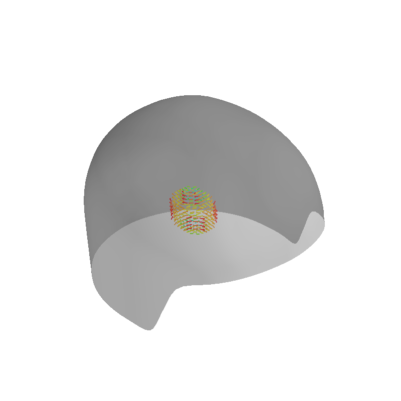
Example showing a gradient coil designed on the surface of a MEG system helmet

import numpy as np
from mayavi import mlab

from bfieldtools.mesh_conductor import MeshConductor
from bfieldtools.coil_optimize import optimize_streamfunctions
from bfieldtools.utils import load_example_mesh
from bfieldtools import sphtools


# Load simple plane mesh that is centered on the origin
helmetmesh = load_example_mesh("meg_helmet")
coil = MeshConductor(mesh_obj=helmetmesh, fix_normals=True)

Set up target and stray field points. Here, the target points are on a volumetric grid within a sphere

offset = np.array([0, 0, 0.04])
center = offset

sidelength = 0.05
n = 12
xx = np.linspace(-sidelength / 2, sidelength / 2, n)
yy = np.linspace(-sidelength / 2, sidelength / 2, n)
zz = np.linspace(-sidelength / 2, sidelength / 2, n)
X, Y, Z = np.meshgrid(xx, yy, zz, indexing="ij")

x = X.ravel()
y = Y.ravel()
z = Z.ravel()

target_points = np.array([x, y, z]).T

# Turn cube into sphere by rejecting points "in the corners"
# and inner points
target_points = (
    target_points[
        (np.linalg.norm(target_points, axis=1) < sidelength / 2)
        * (np.linalg.norm(target_points, axis=1) > sidelength / 2 * 0.8)
    ]
    + center
)

Specify target field and run solver. Here, we specify the target field through the use of spherical harmonics. We want to produce the field corresponding to a specific beta_l,m-component.

lmax = 3
alm = np.zeros((lmax * (lmax + 2),))
blm = np.zeros((lmax * (lmax + 2),))

# Set one specific component to one
blm[3] += 1

sphfield = sphtools.field(target_points, alm, blm, lmax)

target_field = sphfield / np.max(sphfield[:, 0])

target_field[:, 2] = 0

coil.plot_mesh(opacity=0.5)
mlab.quiver3d(*target_points.T, *sphfield.T)
mlab.gcf().scene.isometric_view()

abs_error = np.zeros_like(target_field)
abs_error[:, 0] += 0.05
abs_error[:, 1:3] += 0.1


target_spec = {
    "coupling": coil.B_coupling(target_points),
    "abs_error": abs_error,
    "target": target_field,
}

Out:

Computing magnetic field coupling matrix, 2044 vertices by 312 target points... took 0.24 seconds.

import mosek

coil.s, prob = optimize_streamfunctions(
    coil,
    [target_spec],
    objective="minimum_inductive_energy",
    solver="MOSEK",
    solver_opts={"mosek_params": {mosek.iparam.num_threads: 8}},
)

Out:

Computing the inductance matrix...
Computing self-inductance matrix using rough quadrature (degree=2).              For higher accuracy, set quad_degree to 4 or more.
Estimating 16313 MiB required for 2044 by 2044 vertices...
Computing inductance matrix in 40 chunks (9384 MiB memory free),              when approx_far=True using more chunks is faster...
Computing triangle-coupling matrix
Inductance matrix computation took 7.43 seconds.
Pre-existing problem not passed, creating...
Passing parameters to problem...
Passing problem to solver...


Problem
  Name                   :
  Objective sense        : min
  Type                   : CONIC (conic optimization problem)
  Constraints            : 3819
  Cones                  : 1
  Scalar variables       : 3893
  Matrix variables       : 0
  Integer variables      : 0

Optimizer started.
Problem
  Name                   :
  Objective sense        : min
  Type                   : CONIC (conic optimization problem)
  Constraints            : 3819
  Cones                  : 1
  Scalar variables       : 3893
  Matrix variables       : 0
  Integer variables      : 0

Optimizer  - threads                : 8
Optimizer  - solved problem         : the dual
Optimizer  - Constraints            : 1946
Optimizer  - Cones                  : 1
Optimizer  - Scalar variables       : 3819              conic                  : 1947
Optimizer  - Semi-definite variables: 0                 scalarized             : 0
Factor     - setup time             : 0.28              dense det. time        : 0.00
Factor     - ML order time          : 0.07              GP order time          : 0.00
Factor     - nonzeros before factor : 1.89e+06          after factor           : 1.89e+06
Factor     - dense dim.             : 0                 flops                  : 8.46e+09
ITE PFEAS    DFEAS    GFEAS    PRSTATUS   POBJ              DOBJ              MU       TIME
0   5.6e+02  1.0e+00  2.0e+00  0.00e+00   0.000000000e+00   -1.000000000e+00  1.0e+00  1.40
1   2.4e+02  4.2e-01  1.2e+00  -9.49e-01  6.650619835e+00   6.946913020e+00   4.2e-01  1.63
2   7.7e+01  1.4e-01  6.3e-01  -8.61e-01  6.505864740e+01   6.862857116e+01   1.4e-01  1.82
3   2.3e+01  4.0e-02  2.4e-01  -6.12e-01  2.768754633e+02   2.845399199e+02   4.0e-02  2.02
4   3.1e+00  5.5e-03  2.6e-02  -9.44e-02  6.459947892e+02   6.513630397e+02   5.5e-03  2.22
5   5.7e-01  1.0e-03  2.2e-03  7.38e-01   5.178338127e+02   5.190086016e+02   1.0e-03  2.42
6   2.8e-01  5.0e-04  7.7e-04  9.52e-01   4.445760451e+02   4.451278532e+02   5.0e-04  2.63
7   5.1e-02  9.0e-05  5.1e-05  9.77e-01   3.974604461e+02   3.975340486e+02   9.0e-05  2.88
8   7.3e-03  1.3e-05  2.7e-06  9.95e-01   3.936012105e+02   3.936113968e+02   1.3e-05  3.15
9   1.0e-03  1.8e-06  1.4e-07  9.99e-01   3.928011290e+02   3.928024812e+02   1.8e-06  3.40
10  1.3e-04  2.4e-07  7.1e-09  1.00e+00   3.927465956e+02   3.927467997e+02   2.4e-07  3.60
11  2.6e-05  4.6e-08  5.9e-10  1.00e+00   3.927424767e+02   3.927425160e+02   4.6e-08  3.81
12  3.0e-06  5.3e-09  2.2e-11  1.00e+00   3.927425347e+02   3.927425392e+02   5.3e-09  4.02
13  4.3e-07  7.6e-10  1.2e-12  1.00e+00   3.927425447e+02   3.927425454e+02   7.6e-10  4.23
14  1.7e-07  1.1e-10  2.2e-13  1.00e+00   3.927425461e+02   3.927425438e+02   9.7e-15  4.46
Optimizer terminated. Time: 4.56


Interior-point solution summary
  Problem status  : PRIMAL_AND_DUAL_FEASIBLE
  Solution status : OPTIMAL
  Primal.  obj: 3.9274254609e+02    nrm: 8e+02    Viol.  con: 3e-13    var: 0e+00    cones: 0e+00
  Dual.    obj: 3.9274254381e+02    nrm: 2e+03    Viol.  con: 3e-10    var: 7e-09    cones: 1e-13

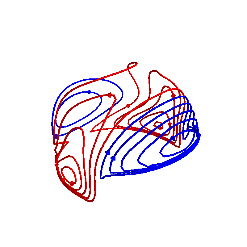
Plot coil windings

loops = coil.s.discretize(N_contours=10)
loops.plot_loops()

Out:

<mayavi.core.scene.Scene object at 0x7f0c11d5cbf0>

Estimated memory usage: 1063 MB