High-order spherical harmonic biplanar coil design

Example showing a basic biplanar coil producing a high-order spherical harmonic field in a specific target region between the two coil planes.

import numpy as np
from mayavi import mlab
import trimesh


from bfieldtools.mesh_conductor import MeshConductor
from bfieldtools.coil_optimize import optimize_streamfunctions
from bfieldtools.utils import combine_meshes, load_example_mesh


# Load simple plane mesh that is centered on the origin
planemesh = load_example_mesh("10x10_plane_hires")

# Specify coil plane geometry
center_offset = np.array([0, 0, 0])
standoff = np.array([0, 3, 0])

# Create coil plane pairs
coil_plus = trimesh.Trimesh(
    planemesh.vertices + center_offset + standoff, planemesh.faces, process=False
)

coil_minus = trimesh.Trimesh(
    planemesh.vertices + center_offset - standoff, planemesh.faces, process=False
)

joined_planes = combine_meshes((coil_plus, coil_minus))

# Create mesh class object
coil = MeshConductor(
    mesh_obj=joined_planes, fix_normals=True, basis_name="suh", N_suh=100
)

Out:

Calculating surface harmonics expansion...
Computing the laplacian matrix...
Computing the mass matrix...

Set up target and stray field points

# Here, the target points are on a volumetric grid within a sphere

center = np.array([0, 0, 0])

sidelength = 1.5
n = 8
xx = np.linspace(-sidelength / 2, sidelength / 2, n)
yy = np.linspace(-sidelength / 2, sidelength / 2, n)
zz = np.linspace(-sidelength / 2, sidelength / 2, n)
X, Y, Z = np.meshgrid(xx, yy, zz, indexing="ij")

x = X.ravel()
y = Y.ravel()
z = Z.ravel()

target_points = np.array([x, y, z]).T

# Turn cube into sphere by rejecting points "in the corners"
target_points = (
    target_points[np.linalg.norm(target_points, axis=1) < sidelength / 2] + center
)

Create bfield specifications used when optimizing the coil geometry

from bfieldtools import sphtools


lmax = 4
alm = np.zeros((lmax * (lmax + 2),))
blm = np.zeros((lmax * (lmax + 2),))

# Set one specific component to one
blm[16] += 1

sphfield = sphtools.field(target_points, alm, blm, lmax)

target_field = sphfield / np.max(sphfield[:, 0])


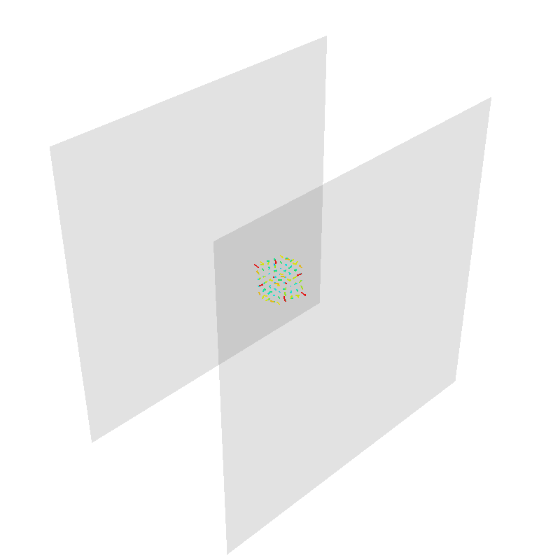
coil.plot_mesh(opacity=0.2)
mlab.quiver3d(*target_points.T, *sphfield.T)


target_spec = {
    "coupling": coil.B_coupling(target_points),
    "abs_error": 0.1,
    "target": target_field,
}

Out:

Computing magnetic field coupling matrix, 3184 vertices by 160 target points... took 0.28 seconds.

Run QP solver

import mosek

coil.s, prob = optimize_streamfunctions(
    coil,
    [target_spec],
    objective="minimum_inductive_energy",
    solver="MOSEK",
    solver_opts={"mosek_params": {mosek.iparam.num_threads: 8}},
)

Out:

Computing the inductance matrix...
Computing self-inductance matrix using rough quadrature (degree=2).              For higher accuracy, set quad_degree to 4 or more.
Estimating 34964 MiB required for 3184 by 3184 vertices...
Computing inductance matrix in 80 chunks (9346 MiB memory free),              when approx_far=True using more chunks is faster...
Computing triangle-coupling matrix
Inductance matrix computation took 13.92 seconds.
Pre-existing problem not passed, creating...
Passing parameters to problem...
Passing problem to solver...


Problem
  Name                   :
  Objective sense        : min
  Type                   : CONIC (conic optimization problem)
  Constraints            : 1062
  Cones                  : 1
  Scalar variables       : 203
  Matrix variables       : 0
  Integer variables      : 0

Optimizer started.
Problem
  Name                   :
  Objective sense        : min
  Type                   : CONIC (conic optimization problem)
  Constraints            : 1062
  Cones                  : 1
  Scalar variables       : 203
  Matrix variables       : 0
  Integer variables      : 0

Optimizer  - threads                : 8
Optimizer  - solved problem         : the dual
Optimizer  - Constraints            : 101
Optimizer  - Cones                  : 1
Optimizer  - Scalar variables       : 646               conic                  : 102
Optimizer  - Semi-definite variables: 0                 scalarized             : 0
Factor     - setup time             : 0.00              dense det. time        : 0.00
Factor     - ML order time          : 0.00              GP order time          : 0.00
Factor     - nonzeros before factor : 5151              after factor           : 5151
Factor     - dense dim.             : 0                 flops                  : 3.56e+06
ITE PFEAS    DFEAS    GFEAS    PRSTATUS   POBJ              DOBJ              MU       TIME
0   8.6e+01  1.0e+00  2.0e+00  0.00e+00   0.000000000e+00   -1.000000000e+00  1.0e+00  0.02
1   2.5e+01  2.9e-01  1.1e+00  -9.80e-01  6.602857671e+00   7.967580453e+00   2.9e-01  0.03
2   8.8e+00  1.0e-01  6.2e-01  -9.80e-01  5.239303076e+01   5.985574557e+01   1.0e-01  0.03
3   6.6e+00  7.6e-02  5.3e-01  -9.41e-01  3.083167508e+02   3.182910044e+02   7.6e-02  0.03
4   1.7e+00  2.0e-02  2.7e-01  -9.69e-01  3.330852315e+02   3.781060675e+02   2.0e-02  0.03
5   7.8e-01  9.0e-03  1.6e-01  -9.34e-01  5.326287527e+03   5.406871451e+03   9.0e-03  0.04
6   1.2e-01  1.3e-03  5.2e-02  -8.38e-01  3.039879998e+04   3.076981322e+04   1.3e-03  0.04
7   3.7e-02  4.3e-04  2.1e-02  -6.09e-01  9.514761096e+04   9.573840935e+04   4.3e-04  0.04
8   5.1e-03  6.0e-05  1.7e-03  -5.30e-02  2.781541372e+05   2.783662751e+05   6.0e-05  0.04
9   4.2e-04  4.9e-06  3.8e-05  1.02e+00   3.269725926e+05   3.269874901e+05   4.9e-06  0.04
10  4.1e-05  4.7e-07  1.4e-06  9.95e-01   3.319026080e+05   3.319042217e+05   4.7e-07  0.05
11  6.3e-06  1.5e-07  8.4e-08  1.00e+00   3.323819910e+05   3.323822412e+05   7.4e-08  0.05
12  3.3e-07  7.5e-09  4.1e-09  1.00e+00   3.324644586e+05   3.324644714e+05   3.8e-09  0.05
13  2.2e-07  4.2e-09  2.0e-09  1.00e+00   3.324664412e+05   3.324664483e+05   2.1e-09  0.06
14  4.1e-07  2.3e-09  5.9e-10  1.00e+00   3.324675822e+05   3.324675861e+05   1.1e-09  0.06
15  4.1e-07  2.3e-09  5.9e-10  1.00e+00   3.324675822e+05   3.324675861e+05   1.1e-09  0.06
16  4.1e-07  2.3e-09  5.9e-10  1.00e+00   3.324675822e+05   3.324675861e+05   1.1e-09  0.07
17  5.1e-07  2.0e-09  3.9e-10  1.00e+00   3.324677418e+05   3.324677452e+05   1.0e-09  0.07
18  5.1e-07  2.0e-09  3.9e-10  1.00e+00   3.324677418e+05   3.324677452e+05   1.0e-09  0.08
19  5.1e-07  2.0e-09  3.9e-10  1.00e+00   3.324677418e+05   3.324677452e+05   1.0e-09  0.08
20  5.3e-07  1.9e-09  1.2e-10  1.00e+00   3.324677771e+05   3.324677805e+05   9.8e-10  0.09
21  5.3e-07  1.9e-09  1.2e-10  1.00e+00   3.324677771e+05   3.324677805e+05   9.8e-10  0.09
Optimizer terminated. Time: 0.10


Interior-point solution summary
  Problem status  : PRIMAL_AND_DUAL_FEASIBLE
  Solution status : OPTIMAL
  Primal.  obj: 3.3246777714e+05    nrm: 7e+05    Viol.  con: 2e-06    var: 0e+00    cones: 0e+00
  Dual.    obj: 3.3246778047e+05    nrm: 4e+05    Viol.  con: 0e+00    var: 7e-06    cones: 0e+00

Plot coil windings and target points

coil.s.discretize(N_contours=10).plot_loops()

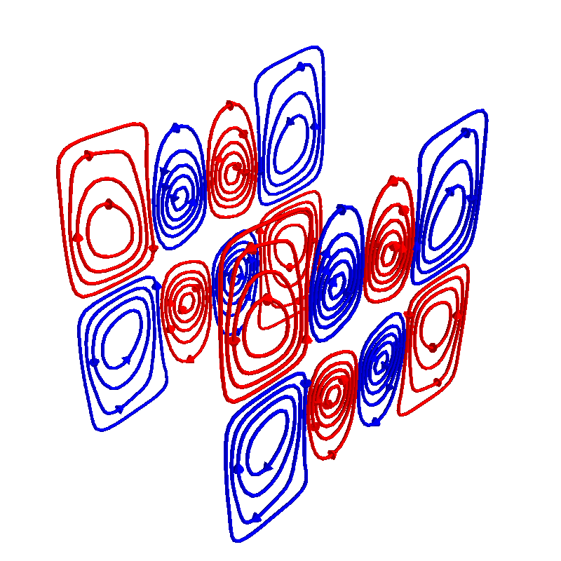
Out:

<mayavi.core.scene.Scene object at 0x7f0c5936c6b0>

Estimated memory usage: 1860 MB