Note
Click here to download the full example code
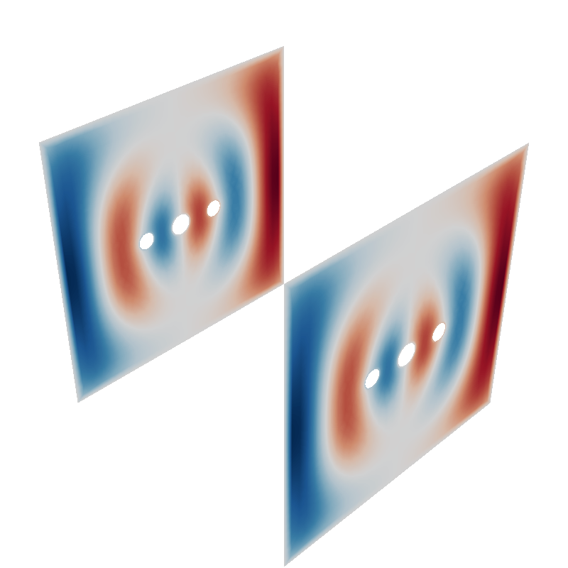
Coil with interior holes
Example showing a basic biplanar coil producing homogeneous field in a target region between the two coil planes. The coil planes have holes in them,
import numpy as np
import trimesh

from bfieldtools.mesh_conductor import MeshConductor
from bfieldtools.coil_optimize import optimize_streamfunctions
from bfieldtools.utils import combine_meshes, load_example_mesh


# Load simple plane mesh that is centered on the origin
planemesh = load_example_mesh("plane_w_holes")

angle = np.pi / 2
rotation_matrix = np.array(
    [
        [1, 0, 0, 0],
        [0, np.cos(angle), -np.sin(angle), 0],
        [0, np.sin(angle), np.cos(angle), 0],
        [0, 0, 0, 1],
    ]
)

planemesh.apply_transform(rotation_matrix)

# Specify coil plane geometry
center_offset = np.array([0, 0, 0])
standoff = np.array([0, 20, 0])

# Create coil plane pairs
coil_plus = trimesh.Trimesh(
    planemesh.vertices + center_offset + standoff, planemesh.faces, process=False
)

coil_minus = trimesh.Trimesh(
    planemesh.vertices + center_offset - standoff, planemesh.faces, process=False
)

joined_planes = combine_meshes((coil_plus, coil_minus))

# Create MeshConductor object, which finds the holes and sets the boundary condition
coil = MeshConductor(mesh_obj=joined_planes, fix_normals=True)
Set up target and stray field points
# Here, the target points are on a volumetric grid within a sphere

center = np.array([0, 0, 0])

sidelength = 10
n = 8
xx = np.linspace(-sidelength / 2, sidelength / 2, n)
yy = np.linspace(-sidelength / 2, sidelength / 2, n)
zz = np.linspace(-sidelength / 2, sidelength / 2, n)
X, Y, Z = np.meshgrid(xx, yy, zz, indexing="ij")

x = X.ravel()
y = Y.ravel()
z = Z.ravel()

target_points = np.array([x, y, z]).T

# Turn cube into sphere by rejecting points "in the corners"
target_points = (
    target_points[np.linalg.norm(target_points, axis=1) < sidelength / 2] + center
)
Create bfield specifications used when optimizing the coil geometry
# The absolute target field amplitude is not of importance,
# and it is scaled to match the C matrix in the optimization function

target_field = np.zeros(target_points.shape)
target_field[:, 0] = target_field[:, 0] + 1

target_abs_error = np.zeros_like(target_field)
target_abs_error[:, 0] += 0.001
target_abs_error[:, 1:3] += 0.005

target_spec = {
    "coupling": coil.B_coupling(target_points),
    "abs_error": target_abs_error,
    "target": target_field,
}

bfield_specification = [target_spec]
Out:
Computing magnetic field coupling matrix, 2772 vertices by 160 target points... took 0.22 seconds.
Run QP solver
import mosek

coil.s, prob = optimize_streamfunctions(
    coil,
    bfield_specification,
    objective="minimum_inductive_energy",
    solver="MOSEK",
    solver_opts={"mosek_params": {mosek.iparam.num_threads: 8}},
)
Out:
Computing the inductance matrix...
Computing self-inductance matrix using rough quadrature (degree=2).              For higher accuracy, set quad_degree to 4 or more.
Estimating 27549 MiB required for 2772 by 2772 vertices...
Computing inductance matrix in 60 chunks (9360 MiB memory free),              when approx_far=True using more chunks is faster...
Computing triangle-coupling matrix
Inductance matrix computation took 10.45 seconds.
Pre-existing problem not passed, creating...
Passing parameters to problem...
Passing problem to solver...


Problem
  Name                   :
  Objective sense        : min
  Type                   : CONIC (conic optimization problem)
  Constraints            : 3364
  Cones                  : 1
  Scalar variables       : 4807
  Matrix variables       : 0
  Integer variables      : 0

Optimizer started.
Problem
  Name                   :
  Objective sense        : min
  Type                   : CONIC (conic optimization problem)
  Constraints            : 3364
  Cones                  : 1
  Scalar variables       : 4807
  Matrix variables       : 0
  Integer variables      : 0

Optimizer  - threads                : 8
Optimizer  - solved problem         : the dual
Optimizer  - Constraints            : 2403
Optimizer  - Cones                  : 1
Optimizer  - Scalar variables       : 3364              conic                  : 2404
Optimizer  - Semi-definite variables: 0                 scalarized             : 0
Factor     - setup time             : 0.34              dense det. time        : 0.00
Factor     - ML order time          : 0.12              GP order time          : 0.00
Factor     - nonzeros before factor : 2.89e+06          after factor           : 2.89e+06
Factor     - dense dim.             : 0                 flops                  : 1.20e+10
ITE PFEAS    DFEAS    GFEAS    PRSTATUS   POBJ              DOBJ              MU       TIME
0   2.6e+02  1.0e+00  2.0e+00  0.00e+00   0.000000000e+00   -1.000000000e+00  1.0e+00  1.40
1   9.5e+01  3.7e-01  3.7e-01  2.72e-01   2.032550662e+01   1.978947626e+01   3.7e-01  1.70
2   5.2e+01  2.0e-01  2.2e-01  2.64e-01   4.206360188e+01   4.172428917e+01   2.0e-01  1.99
3   2.1e+01  8.1e-02  3.1e-02  1.43e+00   9.031259720e+01   9.017883545e+01   8.1e-02  2.29
4   8.3e+00  3.2e-02  1.0e-02  9.42e-01   9.954558419e+01   9.949694972e+01   3.2e-02  2.56
5   7.6e-01  3.0e-03  3.5e-04  9.78e-01   1.076262176e+02   1.076229362e+02   3.0e-03  2.93
6   1.0e-01  4.0e-04  1.8e-05  1.02e+00   1.086072215e+02   1.086067963e+02   4.0e-04  3.27
7   1.4e-02  5.4e-05  9.0e-07  1.00e+00   1.087762905e+02   1.087762356e+02   5.4e-05  3.60
8   2.2e-03  8.4e-06  5.5e-08  1.00e+00   1.087997220e+02   1.087997135e+02   8.4e-06  3.91
9   1.9e-04  7.5e-07  1.4e-09  1.00e+00   1.088036087e+02   1.088036080e+02   7.5e-07  4.26
10  9.3e-05  3.6e-07  5.0e-10  1.00e+00   1.088037954e+02   1.088037951e+02   3.6e-07  4.59
11  1.3e-05  4.9e-08  2.2e-11  1.00e+00   1.088039483e+02   1.088039483e+02   4.9e-08  4.91
12  2.5e-06  9.6e-09  3.7e-11  1.00e+00   1.088039680e+02   1.088039683e+02   9.6e-09  5.21
13  5.0e-07  2.0e-09  3.0e-12  1.00e+00   1.088039719e+02   1.088039720e+02   2.0e-09  5.69
Optimizer terminated. Time: 5.78


Interior-point solution summary
  Problem status  : PRIMAL_AND_DUAL_FEASIBLE
  Solution status : OPTIMAL
  Primal.  obj: 1.0880397193e+02    nrm: 2e+02    Viol.  con: 2e-09    var: 0e+00    cones: 0e+00
  Dual.    obj: 1.0880397200e+02    nrm: 3e+03    Viol.  con: 1e-07    var: 2e-09    cones: 0e+00
Plot the computed streamfunction
coil.s.plot(ncolors=256)
Out:
<mayavi.modules.surface.Surface object at 0x7f0bf97d1230>
Total running time of the script: ( 0 minutes 21.910 seconds)
Estimated memory usage: 1437 MB