Note
Click here to download the full example code
Spherical harmonics-generating coil design
Example showing a basic biplanar coil producing a field profile defined by spherical harmonics. We use the surface harmonics basis for the stream function, and optimize the coupling to spherical harmonics components, thus creating a compact optimization problem that can be solved very quickly.
import numpy as np
import trimesh

from bfieldtools.mesh_conductor import MeshConductor
from bfieldtools.coil_optimize import optimize_streamfunctions
from bfieldtools.utils import combine_meshes, load_example_mesh


# Load simple plane mesh that is centered on the origin
planemesh = load_example_mesh("10x10_plane_hires")

# Specify coil plane geometry
center_offset = np.array([0, 0, 0])
standoff = np.array([0, 15, 0])

# Create coil plane pairs
coil_plus = trimesh.Trimesh(
    planemesh.vertices + center_offset + standoff, planemesh.faces, process=False
)

coil_minus = trimesh.Trimesh(
    planemesh.vertices + center_offset - standoff, planemesh.faces, process=False
)

joined_planes = combine_meshes((coil_plus, coil_minus))


# To spice things up, let's distort the planes a bit
joined_planes.vertices = (
    joined_planes.vertices
    - 0.5
    * np.linalg.norm(joined_planes.vertices, axis=1)[:, None]
    * np.sign(joined_planes.vertices[:, 1])[:, None]
    * joined_planes.vertex_normals
)

joined_planes.vertices = (
    joined_planes.vertices
    - 0.5
    * np.linalg.norm(joined_planes.vertices, axis=1)[:, None]
    * np.sign(joined_planes.vertices[:, 1])[:, None]
    * joined_planes.vertex_normals
)


# Create mesh class object
coil = MeshConductor(
    mesh_obj=joined_planes,
    fix_normals=True,
    basis_name="suh",
    N_suh=100,
    sph_radius=0.2,
    sph_normalization="energy",
)
Out:
Calculating surface harmonics expansion...
Computing the laplacian matrix...
Computing the mass matrix...
Set up target spherical harmonics components
target_alms = np.zeros((coil.opts["N_sph"] * (coil.opts["N_sph"] + 2),))
target_blms = np.zeros((coil.opts["N_sph"] * (coil.opts["N_sph"] + 2),))

target_blms[4] += 1
Create bfield specifications used when optimizing the coil geometry
target_spec = {
    "coupling": coil.sph_couplings[1],
    "abs_error": 0.01,
    "target": target_blms,
}
Out:
Computing coupling matrices
l = 1 computed
l = 2 computed
l = 3 computed
l = 4 computed
l = 5 computed
Run QP solver
import mosek

coil.s, prob = optimize_streamfunctions(
    coil,
    [target_spec],
    objective="minimum_ohmic_power",
    solver="MOSEK",
    solver_opts={"mosek_params": {mosek.iparam.num_threads: 8}},
)
Out:
Computing the resistance matrix...
Pre-existing problem not passed, creating...
Passing parameters to problem...
Passing problem to solver...


Problem
  Name                   :
  Objective sense        : min
  Type                   : CONIC (conic optimization problem)
  Constraints            : 172
  Cones                  : 1
  Scalar variables       : 203
  Matrix variables       : 0
  Integer variables      : 0

Optimizer started.
Problem
  Name                   :
  Objective sense        : min
  Type                   : CONIC (conic optimization problem)
  Constraints            : 172
  Cones                  : 1
  Scalar variables       : 203
  Matrix variables       : 0
  Integer variables      : 0

Optimizer  - threads                : 8
Optimizer  - solved problem         : the primal
Optimizer  - Constraints            : 21
Optimizer  - Cones                  : 1
Optimizer  - Scalar variables       : 122               conic                  : 102
Optimizer  - Semi-definite variables: 0                 scalarized             : 0
Factor     - setup time             : 0.00              dense det. time        : 0.00
Factor     - ML order time          : 0.00              GP order time          : 0.00
Factor     - nonzeros before factor : 231               after factor           : 231
Factor     - dense dim.             : 0                 flops                  : 4.57e+04
ITE PFEAS    DFEAS    GFEAS    PRSTATUS   POBJ              DOBJ              MU       TIME
0   2.6e+03  1.0e+00  1.0e+00  0.00e+00   5.000000000e-01   5.000000000e-01   1.0e+00  0.00
1   3.5e+02  1.3e-01  3.6e-01  -9.99e-01  2.106776004e+00   8.539033584e+00   1.3e-01  0.00
2   5.9e+01  2.2e-02  1.4e-01  -9.86e-01  1.056154434e+01   5.043072723e+01   2.2e-02  0.01
3   7.2e+00  2.7e-03  3.9e-02  -8.86e-01  5.862068212e+01   2.665291713e+02   2.7e-03  0.01
4   9.5e-01  3.6e-04  4.7e-03  -1.93e-01  7.820100570e+01   2.457313707e+02   3.6e-04  0.01
5   7.1e-02  2.7e-05  8.2e-05  8.62e-01   1.581261876e+01   2.492473364e+01   2.7e-05  0.01
6   3.1e-03  1.2e-06  6.1e-07  1.12e+00   1.293685796e+01   1.320298909e+01   1.2e-06  0.01
7   2.7e-04  1.0e-07  1.5e-08  1.10e+00   1.268464223e+01   1.270457442e+01   1.0e-07  0.01
8   7.9e-07  3.0e-10  2.1e-12  1.01e+00   1.260896786e+01   1.260901454e+01   3.0e-10  0.01
9   5.5e-10  2.8e-13  8.2e-18  1.00e+00   1.260893219e+01   1.260893222e+01   2.1e-13  0.01
Optimizer terminated. Time: 0.01


Interior-point solution summary
  Problem status  : PRIMAL_AND_DUAL_FEASIBLE
  Solution status : OPTIMAL
  Primal.  obj: 1.2608932191e+01    nrm: 3e+01    Viol.  con: 1e-10    var: 0e+00    cones: 0e+00
  Dual.    obj: 1.2608932224e+01    nrm: 3e+01    Viol.  con: 2e-05    var: 1e-11    cones: 0e+00
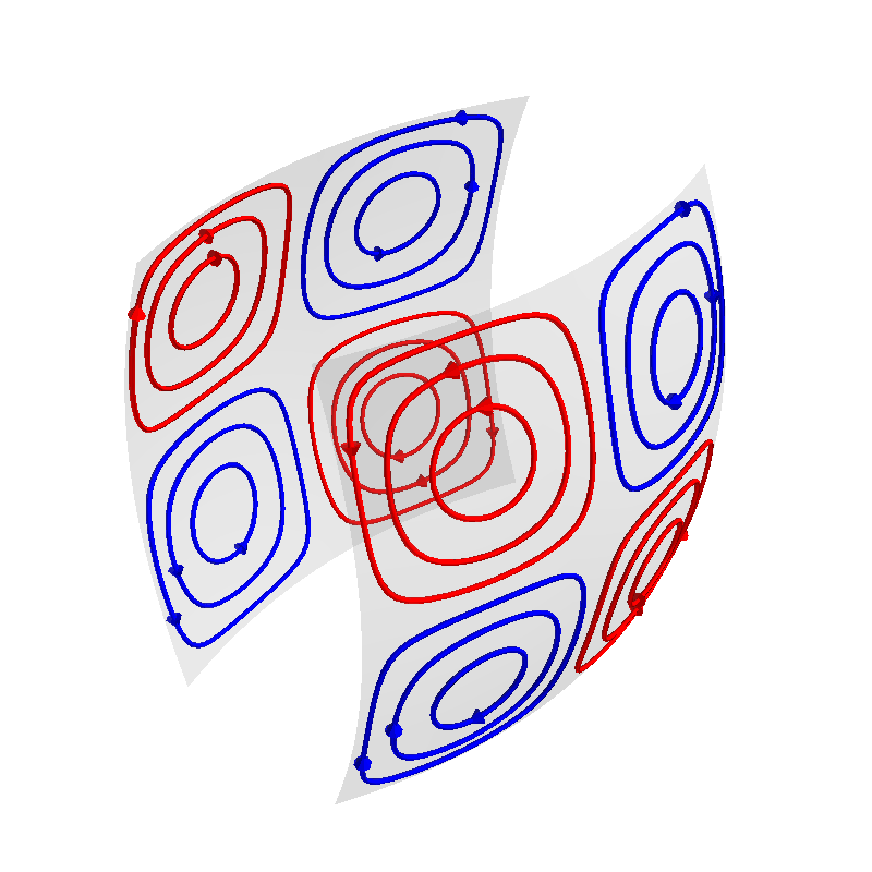
Plot coil windings
f = coil.plot_mesh(opacity=0.2)

loops = coil.s.discretize(N_contours=6)

loops.plot_loops(figure=f)
Out:
<mayavi.core.scene.Scene object at 0x7fa450fab8f0>
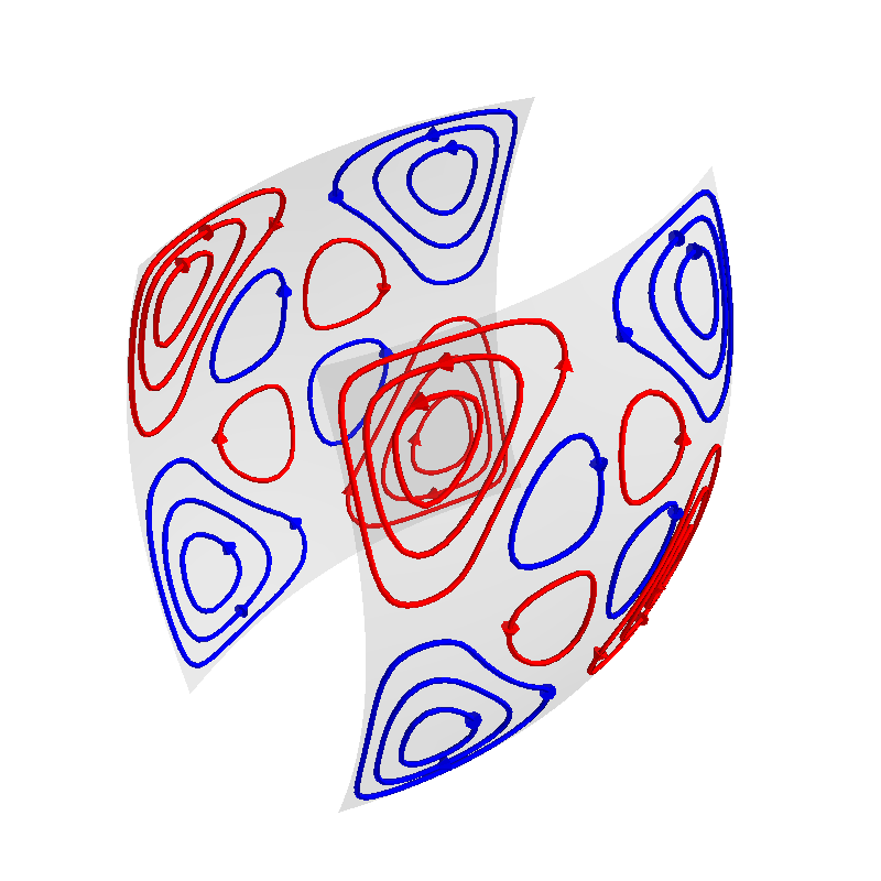
Now, let’s change the spherical harmonics inner expansion radius (i.e. the target region radius) and optimize a new coil (with the same target sph component)
coil.set_sph_options(sph_radius=1.4)


target_spec = {
    "coupling": coil.sph_couplings[1],
    "abs_error": 0.01,
    "target": target_blms,
}
Out:
Computing coupling matrices
l = 1 computed
l = 2 computed
l = 3 computed
l = 4 computed
l = 5 computed
Run QP solver
import mosek

coil.s2, prob = optimize_streamfunctions(
    coil,
    [target_spec],
    objective="minimum_ohmic_power",
    solver="MOSEK",
    solver_opts={"mosek_params": {mosek.iparam.num_threads: 8}},
)
Out:
Pre-existing problem not passed, creating...
Passing parameters to problem...
Passing problem to solver...


Problem
  Name                   :
  Objective sense        : min
  Type                   : CONIC (conic optimization problem)
  Constraints            : 172
  Cones                  : 1
  Scalar variables       : 203
  Matrix variables       : 0
  Integer variables      : 0

Optimizer started.
Problem
  Name                   :
  Objective sense        : min
  Type                   : CONIC (conic optimization problem)
  Constraints            : 172
  Cones                  : 1
  Scalar variables       : 203
  Matrix variables       : 0
  Integer variables      : 0

Optimizer  - threads                : 8
Optimizer  - solved problem         : the primal
Optimizer  - Constraints            : 21
Optimizer  - Cones                  : 1
Optimizer  - Scalar variables       : 122               conic                  : 102
Optimizer  - Semi-definite variables: 0                 scalarized             : 0
Factor     - setup time             : 0.00              dense det. time        : 0.00
Factor     - ML order time          : 0.00              GP order time          : 0.00
Factor     - nonzeros before factor : 231               after factor           : 231
Factor     - dense dim.             : 0                 flops                  : 4.58e+04
ITE PFEAS    DFEAS    GFEAS    PRSTATUS   POBJ              DOBJ              MU       TIME
0   2.0e+00  1.0e+00  1.0e+00  0.00e+00   5.000000000e-01   5.000000000e-01   1.0e+00  0.00
1   6.7e-01  3.3e-01  1.8e-01  1.14e+00   3.511690623e-01   3.232903157e-01   3.3e-01  0.01
2   2.5e-01  1.3e-01  1.9e-02  9.73e-01   1.001501457e+00   9.333696466e-01   1.3e-01  0.01
3   3.9e-02  2.0e-02  6.8e-04  1.31e+00   1.073643030e+00   1.063449217e+00   2.0e-02  0.01
4   4.2e-03  2.1e-03  2.2e-05  1.32e+00   1.085794962e+00   1.084873799e+00   2.1e-03  0.01
5   7.5e-05  3.8e-05  4.8e-08  1.21e+00   1.088222840e+00   1.088208156e+00   3.8e-05  0.01
6   1.5e-07  7.5e-08  4.3e-12  1.01e+00   1.088267709e+00   1.088267680e+00   7.5e-08  0.01
7   5.8e-10  1.4e-10  1.2e-15  1.00e+00   1.088267811e+00   1.088267811e+00   2.9e-10  0.01
Optimizer terminated. Time: 0.01


Interior-point solution summary
  Problem status  : PRIMAL_AND_DUAL_FEASIBLE
  Solution status : OPTIMAL
  Primal.  obj: 1.0882678108e+00    nrm: 4e+00    Viol.  con: 2e-10    var: 0e+00    cones: 0e+00
  Dual.    obj: 1.0882678106e+00    nrm: 9e+00    Viol.  con: 2e-08    var: 6e-11    cones: 0e+00
Plot coil windings
f2 = coil.plot_mesh(opacity=0.2)

loops2 = coil.s2.discretize(N_contours=6)

loops2.plot_loops(figure=f2)
Out:
<mayavi.core.scene.Scene object at 0x7fa4369149b0>
Total running time of the script: ( 0 minutes 46.518 seconds)
Estimated memory usage: 262 MB