Note
Click here to download the full example code
MAMBA coil
Compact example of a biplanar coil producing homogeneous field in a number of target regions arranged in a grid. Meant to demonstrate the flexibility in target choice, inspired by the technique “multiple-acquisition micro B(0) array” (MAMBA) technique, see https://doi.org/10.1002/mrm.10464
import numpy as np
from mayavi import mlab
import trimesh


from bfieldtools.mesh_conductor import MeshConductor
from bfieldtools.coil_optimize import optimize_streamfunctions
from bfieldtools.contour import scalar_contour
from bfieldtools.viz import plot_3d_current_loops

from bfieldtools.utils import combine_meshes, load_example_mesh


# Load simple plane mesh that is centered on the origin
planemesh = load_example_mesh("10x10_plane_hires")

# Specify coil plane geometry
center_offset = np.array([0, 0, 0])
standoff = np.array([0, 1.5, 0])

# Create coil plane pairs
coil_plus = trimesh.Trimesh(
    planemesh.vertices + center_offset + standoff, planemesh.faces, process=False
)

coil_minus = trimesh.Trimesh(
    planemesh.vertices + center_offset - standoff, planemesh.faces, process=False
)

joined_planes = combine_meshes((coil_plus, coil_minus))

# Create mesh class object
coil = MeshConductor(mesh_obj=joined_planes, fix_normals=True, basis_name="inner")
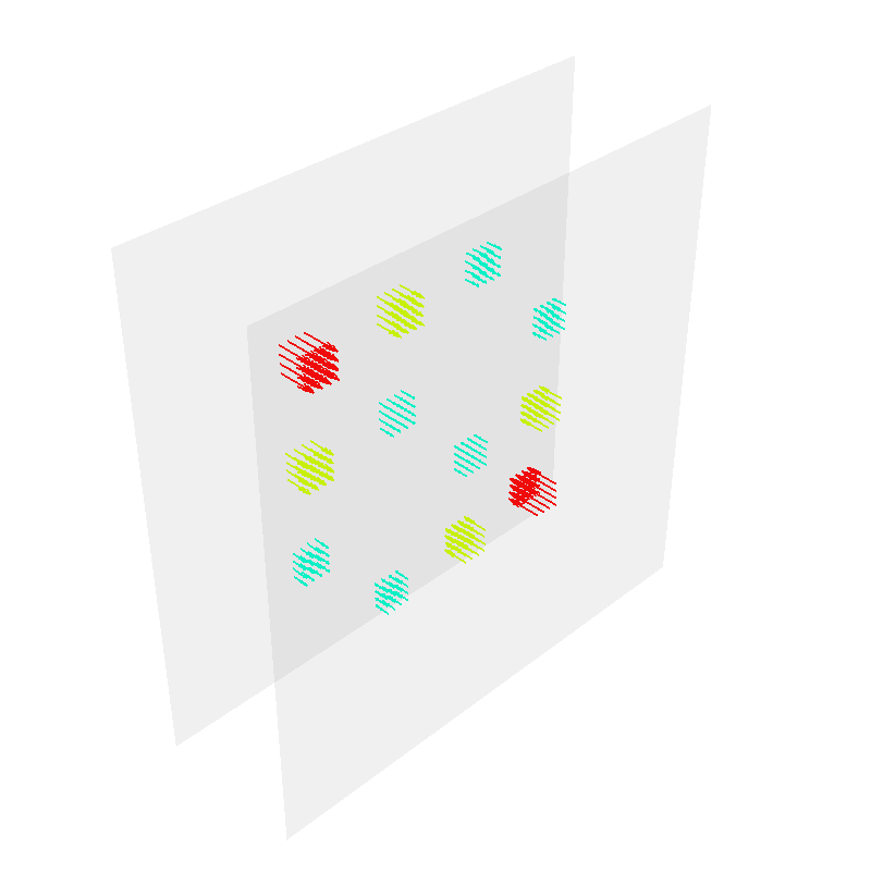
Set up target and stray field points. Here, the target points are on a planar 4x4 grid slightly smaller than the coil dimensions.
center = np.array([0, 0, 0])

sidelength = 0.5
n = 4

height = 0.1
n_height = 2
xx = np.linspace(-sidelength / 2, sidelength / 2, n)
yy = np.linspace(-height / 2, height / 2, n_height)
zz = np.linspace(-sidelength / 2, sidelength / 2, n)
X, Y, Z = np.meshgrid(xx, yy, zz, indexing="ij")

x = X.ravel()
y = Y.ravel()
z = Z.ravel()

target_points = np.array([x, y, z]).T


grid_target_points = list()
target_field = list()

hori_offsets = [-3, -1, 1, 3]
vert_offsets = [-3, -1, 1, 3]

for i, offset_x in enumerate(hori_offsets):
    for j, offset_y in enumerate(vert_offsets):
        grid_target_points.append(target_points + np.array([offset_x, 0, offset_y]))
        target_field.append((i + j - 3) * np.ones((len(target_points),)))

target_points = np.asarray(grid_target_points).reshape((-1, 3))
target_field = np.asarray(target_field).reshape((-1,))

target_field = np.array(
    [np.zeros((len(target_field),)), target_field, np.zeros((len(target_field),))]
).T


target_abs_error = np.zeros_like(target_field)
target_abs_error[:, 1] += 0.1
target_abs_error[:, 0::2] += 0.1
Plot target points and mesh
coil.plot_mesh(opacity=0.1)
mlab.quiver3d(*target_points.T, *target_field.T)
Out:
<mayavi.modules.vectors.Vectors object at 0x7f0c11cf0590>
Compute coupling matrix that is used to compute the generated magnetic field, create field specification
target_spec = {
    "coupling": coil.B_coupling(target_points),
    "abs_error": target_abs_error,
    "target": target_field,
}
Out:
Computing magnetic field coupling matrix, 3184 vertices by 512 target points... took 0.57 seconds.
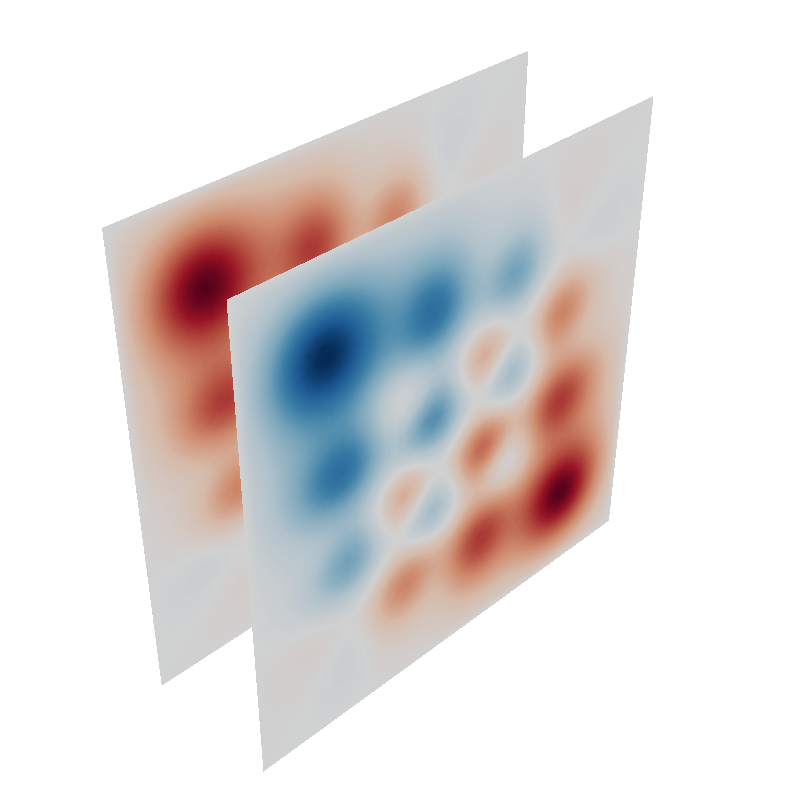
Run QP solver, plot result
import mosek
coil.s, prob = optimize_streamfunctions(
coil,
[target_spec],
objective="minimum_inductive_energy",
solver="MOSEK",
solver_opts={"mosek_params": {mosek.iparam.num_threads: 8}},
)
coil.s.plot()
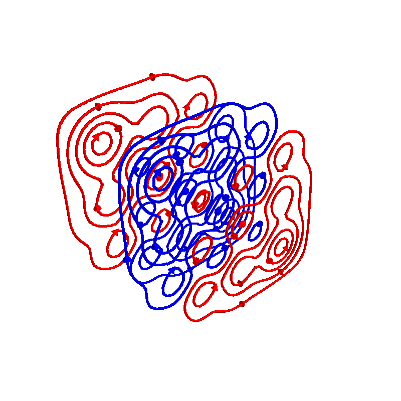
coil.s.discretize(N_contours=10).plot_loops()
Out:
Computing the inductance matrix...
Computing self-inductance matrix using rough quadrature (degree=2).              For higher accuracy, set quad_degree to 4 or more.
Estimating 34964 MiB required for 3184 by 3184 vertices...
Computing inductance matrix in 80 chunks (9273 MiB memory free),              when approx_far=True using more chunks is faster...
Computing triangle-coupling matrix
Inductance matrix computation took 14.08 seconds.
Pre-existing problem not passed, creating...
Passing parameters to problem...
Passing problem to solver...


Problem
  Name                   :
  Objective sense        : min
  Type                   : CONIC (conic optimization problem)
  Constraints            : 5970
  Cones                  : 1
  Scalar variables       : 5795
  Matrix variables       : 0
  Integer variables      : 0

Optimizer started.
Problem
  Name                   :
  Objective sense        : min
  Type                   : CONIC (conic optimization problem)
  Constraints            : 5970
  Cones                  : 1
  Scalar variables       : 5795
  Matrix variables       : 0
  Integer variables      : 0

Optimizer  - threads                : 8
Optimizer  - solved problem         : the dual
Optimizer  - Constraints            : 2897
Optimizer  - Cones                  : 1
Optimizer  - Scalar variables       : 5970              conic                  : 2898
Optimizer  - Semi-definite variables: 0                 scalarized             : 0
Factor     - setup time             : 1.06              dense det. time        : 0.00
Factor     - ML order time          : 0.20              GP order time          : 0.00
Factor     - nonzeros before factor : 4.20e+06          after factor           : 4.20e+06
Factor     - dense dim.             : 0                 flops                  : 2.91e+10
ITE PFEAS    DFEAS    GFEAS    PRSTATUS   POBJ              DOBJ              MU       TIME
0   2.0e+02  1.0e+00  2.0e+00  0.00e+00   0.000000000e+00   -1.000000000e+00  1.0e+00  3.98
1   7.5e+01  3.8e-01  1.1e+00  -8.29e-01  1.092527523e+01   1.122576890e+01   3.8e-01  4.73
2   1.4e+01  7.0e-02  2.7e-01  -5.83e-01  1.310063162e+02   1.338387135e+02   7.0e-02  5.42
3   4.9e-01  2.5e-03  5.1e-03  1.88e-01   2.176256409e+02   2.186500663e+02   2.5e-03  6.06
4   1.0e-01  5.3e-04  3.6e-04  9.63e-01   1.601982077e+02   1.603056738e+02   5.3e-04  6.77
5   8.8e-03  4.4e-05  6.0e-06  9.92e-01   1.504225631e+02   1.504261347e+02   4.4e-05  7.43
6   3.6e-03  1.8e-05  1.6e-06  9.99e-01   1.496646785e+02   1.496661966e+02   1.8e-05  8.15
7   5.0e-04  2.5e-06  8.5e-08  1.00e+00   1.494005013e+02   1.494007311e+02   2.5e-06  8.89
8   2.5e-04  1.3e-06  3.0e-08  1.00e+00   1.493866996e+02   1.493868138e+02   1.3e-06  9.52
9   4.0e-05  2.0e-07  1.9e-09  1.00e+00   1.493759608e+02   1.493759792e+02   2.0e-07  10.14
10  4.8e-06  2.4e-08  8.1e-11  1.00e+00   1.493742426e+02   1.493742448e+02   2.4e-08  10.92
11  7.9e-08  8.7e-11  6.6e-13  1.00e+00   1.493740288e+02   1.493740285e+02   6.2e-12  11.69
Optimizer terminated. Time: 11.95


Interior-point solution summary
  Problem status  : PRIMAL_AND_DUAL_FEASIBLE
  Solution status : OPTIMAL
  Primal.  obj: 1.4937402879e+02    nrm: 3e+02    Viol.  con: 2e-10    var: 0e+00    cones: 0e+00
  Dual.    obj: 1.4937402853e+02    nrm: 7e+01    Viol.  con: 3e-09    var: 1e-09    cones: 0e+00

<mayavi.core.scene.Scene object at 0x7f0c11d5cc50>
Total running time of the script: ( 0 minutes 41.531 seconds)
Estimated memory usage: 2569 MB