Note
Click here to download the full example code
Biplanar coil design
Example showing a basic biplanar coil producing homogeneous field in a target region between the two coil planes.
import numpy as np
import matplotlib.pyplot as plt
from mayavi import mlab
import trimesh


from bfieldtools.mesh_conductor import MeshConductor
from bfieldtools.coil_optimize import optimize_streamfunctions
from bfieldtools.viz import plot_cross_section
from bfieldtools.utils import combine_meshes, load_example_mesh


# Load simple plane mesh that is centered on the origin
planemesh = load_example_mesh("10x10_plane_hires")

# Specify coil plane geometry
center_offset = np.array([0, 0, 0])
standoff = np.array([0, 3, 0])

# Create coil plane pairs
coil_plus = trimesh.Trimesh(
    planemesh.vertices + center_offset + standoff, planemesh.faces, process=False
)

coil_minus = trimesh.Trimesh(
    planemesh.vertices + center_offset - standoff, planemesh.faces, process=False
)

joined_planes = combine_meshes((coil_plus, coil_minus))

# Create mesh class object
coil = MeshConductor(
    mesh_obj=joined_planes, fix_normals=True, basis_name="suh", N_suh=100
)
Out:
Calculating surface harmonics expansion...
Computing the laplacian matrix...
Computing the mass matrix...
Set up target and stray field points
# Here, the target points are on a volumetric grid within a sphere

center = np.array([0, 0, 0])

sidelength = 1.5
n = 8
xx = np.linspace(-sidelength / 2, sidelength / 2, n)
yy = np.linspace(-sidelength / 2, sidelength / 2, n)
zz = np.linspace(-sidelength / 2, sidelength / 2, n)
X, Y, Z = np.meshgrid(xx, yy, zz, indexing="ij")

x = X.ravel()
y = Y.ravel()
z = Z.ravel()

target_points = np.array([x, y, z]).T

# Turn cube into sphere by rejecting points "in the corners"
target_points = (
    target_points[np.linalg.norm(target_points, axis=1) < sidelength / 2] + center
)


# Here, the stray field points are on a spherical surface
stray_radius = 20
stray_points_mesh = trimesh.creation.icosphere(subdivisions=3, radius=stray_radius)
stray_points = stray_points_mesh.vertices + center

n_stray_points = len(stray_points)
Create bfield specifications used when optimizing the coil geometry
# The absolute target field amplitude is not of importance,
# and it is scaled to match the C matrix in the optimization function

target_field = np.zeros(target_points.shape)
target_field[:, 0] += 1

target_spec = {
    "coupling": coil.B_coupling(target_points),
    "abs_error": 0.01,
    "target": target_field,
}
stray_spec = {
    "coupling": coil.B_coupling(stray_points),
    "abs_error": 0.01,
    "target": np.zeros((n_stray_points, 3)),
}

bfield_specification = [target_spec, stray_spec]
Out:
Computing magnetic field coupling matrix, 3184 vertices by 160 target points... took 0.29 seconds.
Computing magnetic field coupling matrix, 3184 vertices by 642 target points... took 0.59 seconds.
# Compute the optimal stream function, either using a numerical solver or regularized least squares
import mosek

coil.s, prob = optimize_streamfunctions(
    coil,
    [target_spec, stray_spec],
    objective="minimum_ohmic_power",
    solver="MOSEK",
    solver_opts={"mosek_params": {mosek.iparam.num_threads: 8}},
)
Out:
Computing the resistance matrix...
Pre-existing problem not passed, creating...
Passing parameters to problem...
Passing problem to solver...


Problem
  Name                   :
  Objective sense        : min
  Type                   : CONIC (conic optimization problem)
  Constraints            : 4914
  Cones                  : 1
  Scalar variables       : 203
  Matrix variables       : 0
  Integer variables      : 0

Optimizer started.
Problem
  Name                   :
  Objective sense        : min
  Type                   : CONIC (conic optimization problem)
  Constraints            : 4914
  Cones                  : 1
  Scalar variables       : 203
  Matrix variables       : 0
  Integer variables      : 0

Optimizer  - threads                : 8
Optimizer  - solved problem         : the dual
Optimizer  - Constraints            : 101
Optimizer  - Cones                  : 1
Optimizer  - Scalar variables       : 2728              conic                  : 102
Optimizer  - Semi-definite variables: 0                 scalarized             : 0
Factor     - setup time             : 0.01              dense det. time        : 0.00
Factor     - ML order time          : 0.00              GP order time          : 0.00
Factor     - nonzeros before factor : 5151              after factor           : 5151
Factor     - dense dim.             : 0                 flops                  : 1.80e+07
ITE PFEAS    DFEAS    GFEAS    PRSTATUS   POBJ              DOBJ              MU       TIME
0   6.6e+02  1.0e+00  2.0e+00  0.00e+00   0.000000000e+00   -1.000000000e+00  1.0e+00  0.09
1   4.4e+02  6.6e-01  1.6e+00  -9.87e-01  1.242404686e-01   -3.791408582e-01  6.6e-01  0.10
2   1.2e+02  1.8e-01  7.8e-01  -9.60e-01  1.109693224e+00   3.956499435e+00   1.8e-01  0.11
3   1.6e+01  2.5e-02  1.8e-01  -7.07e-01  2.865215552e+01   4.020725058e+01   2.5e-02  0.12
4   7.0e-01  1.1e-03  3.6e-03  2.13e-01   3.463100175e+01   3.738850118e+01   1.1e-03  0.12
5   5.4e-01  8.2e-04  2.3e-03  1.20e+00   2.186623490e+01   2.373566156e+01   8.2e-04  0.13
6   4.7e-01  7.1e-04  1.8e-03  1.16e+00   2.672175433e+01   2.827057607e+01   7.1e-04  0.13
7   3.5e-01  5.3e-04  1.1e-03  1.13e+00   1.305976521e+01   1.412810407e+01   5.3e-04  0.14
8   6.6e-02  1.0e-04  7.6e-05  1.09e+00   1.135207342e+01   1.148805971e+01   1.0e-04  0.14
9   4.3e-03  6.5e-06  7.8e-07  1.02e+00   8.889593586e+00   8.892801886e+00   6.5e-06  0.15
10  1.4e-03  2.2e-06  1.5e-07  1.00e+00   8.380254067e+00   8.381363950e+00   2.2e-06  0.16
11  1.1e-04  1.6e-07  3.2e-09  1.00e+00   8.297805381e+00   8.297892684e+00   1.6e-07  0.16
12  4.1e-06  6.2e-09  2.4e-11  1.00e+00   8.294700570e+00   8.294703920e+00   6.2e-09  0.17
13  2.0e-07  3.0e-10  2.5e-13  1.00e+00   8.294657265e+00   8.294657426e+00   3.0e-10  0.18
14  3.0e-09  4.5e-12  1.2e-15  1.00e+00   8.294654536e+00   8.294654538e+00   4.5e-12  0.19
Optimizer terminated. Time: 0.19


Interior-point solution summary
  Problem status  : PRIMAL_AND_DUAL_FEASIBLE
  Solution status : OPTIMAL
  Primal.  obj: 8.2946545357e+00    nrm: 2e+01    Viol.  con: 1e-10    var: 0e+00    cones: 0e+00
  Dual.    obj: 8.2946545378e+00    nrm: 4e+01    Viol.  con: 7e-06    var: 2e-11    cones: 0e+00
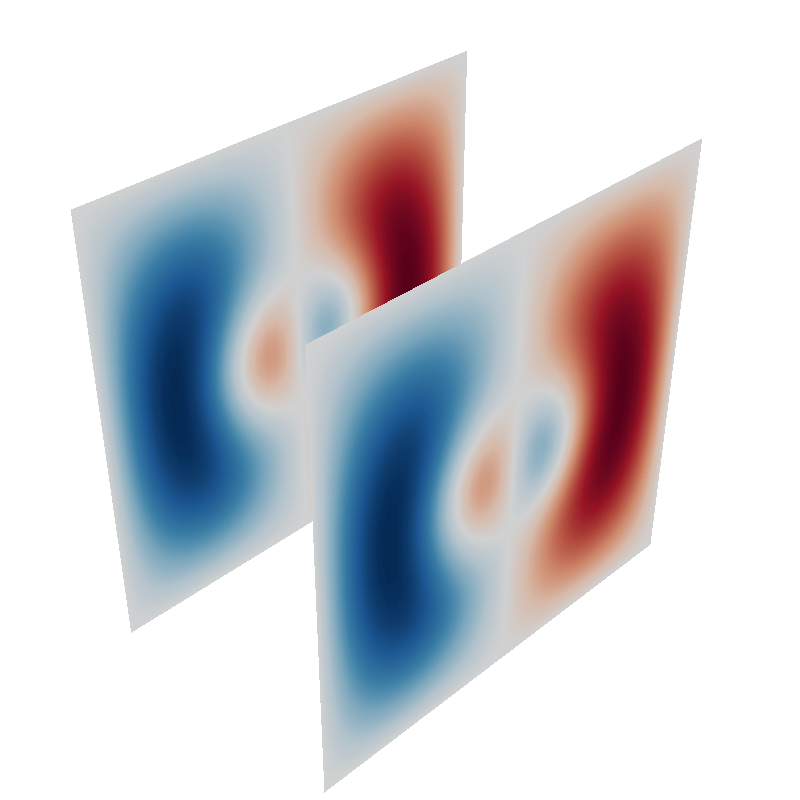
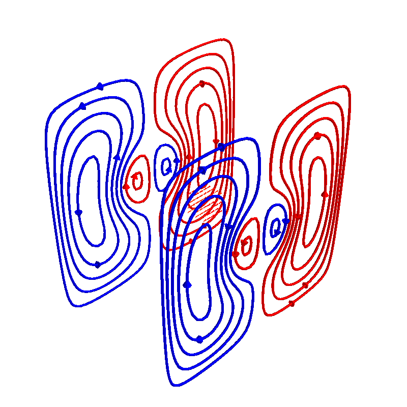
Plot the optimized stream function, then discretize it and plot coil windings and the resultant magnetic field
coil.s.plot()

loops = coil.s.discretize(N_contours=10)

loops.plot_loops()

B_target = loops.magnetic_field(target_points)
mlab.quiver3d(*target_points.T, *B_target.T)
Out:
<mayavi.modules.vectors.Vectors object at 0x7f0c5979a470>
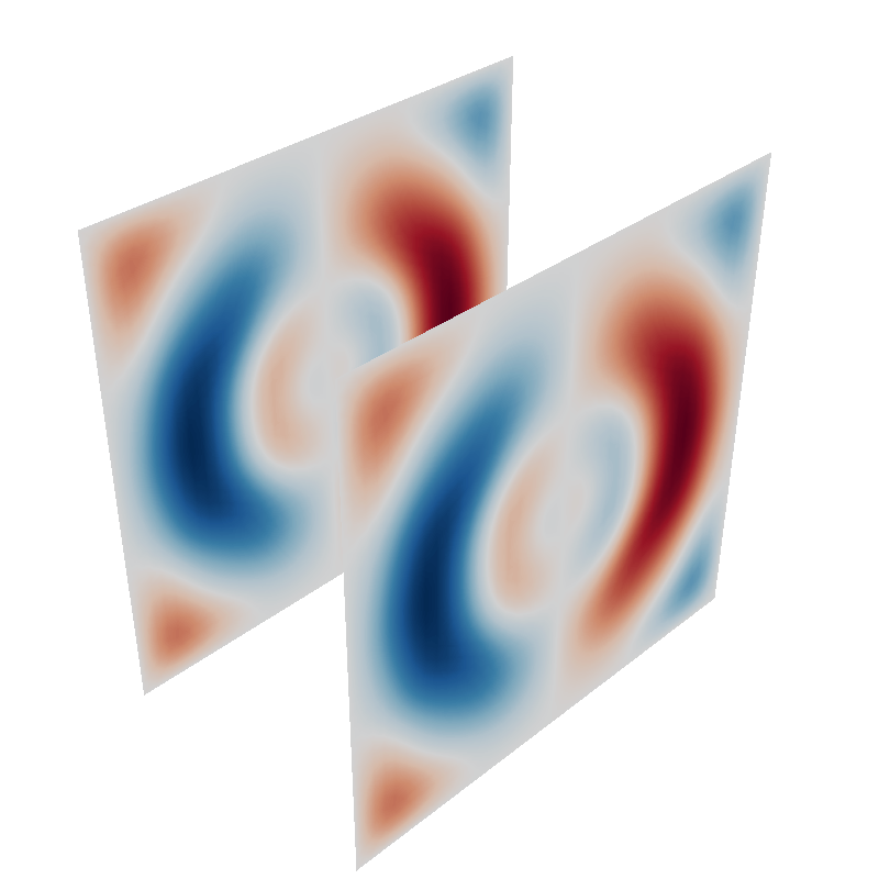
Lets also do the same coil optimization using regularized least-squares. Now we can’t specify inequality constraints (e.g. use error margins in the specification).
from bfieldtools.coil_optimize import optimize_lsq

coil.s2 = optimize_lsq(
    coil, [target_spec, stray_spec], objective="minimum_ohmic_power", reg=1e6
)
Out:
Error tolerances in specification will be ignored when using lsq
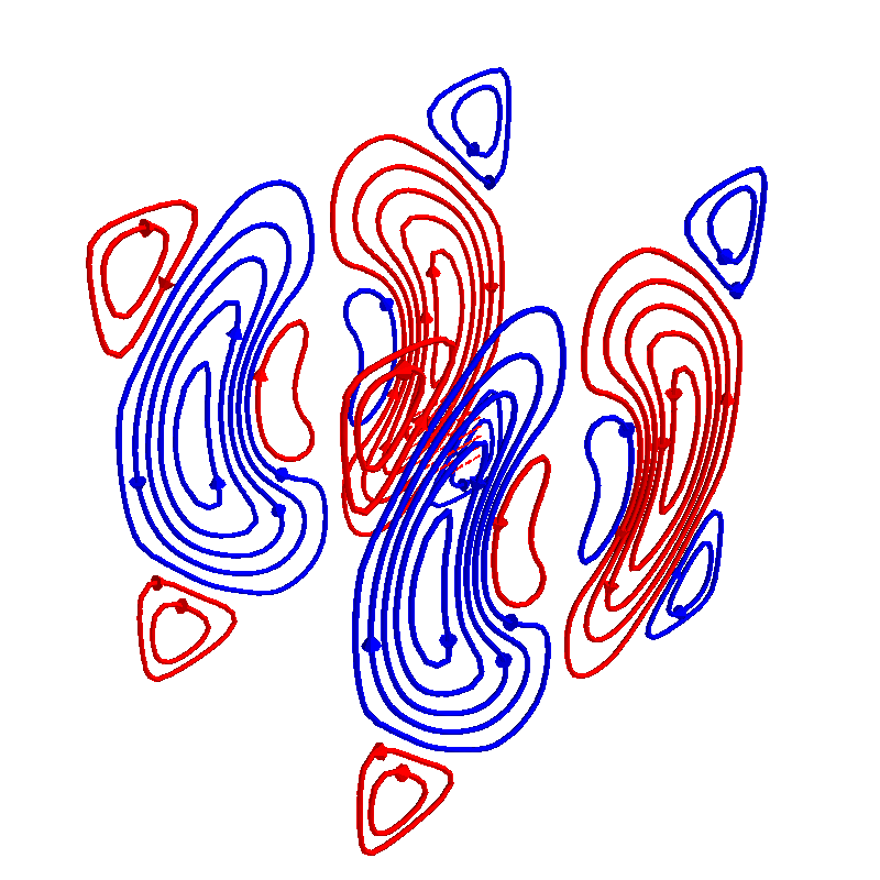
Plot the optimized stream function, then discretize it and plot coil windings and the resultant magnetic field
coil.s2.plot()

loops2 = coil.s2.discretize(N_contours=10)

loops2.plot_loops()

B_target = loops2.magnetic_field(target_points)
mlab.quiver3d(*target_points.T, *B_target.T)
Out:
<mayavi.modules.vectors.Vectors object at 0x7f0c5926ae30>
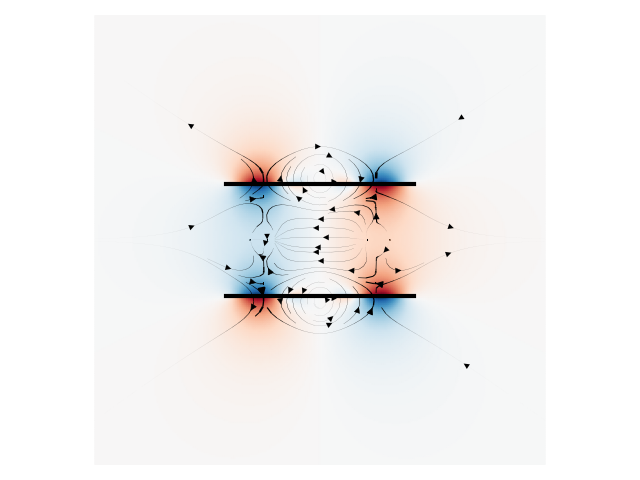
Plot cross-section of magnetic field and magnetic potential of the discretized loops
x = y = np.linspace(-12, 12, 250)
X, Y = np.meshgrid(x, y, indexing="ij")


points = np.zeros((X.flatten().shape[0], 3))
points[:, 0] = X.flatten()
points[:, 1] = Y.flatten()

B = loops2.magnetic_field(points)
U = loops2.scalar_potential(points)

U = U.reshape(x.shape[0], y.shape[0])
B = B.T[:2].reshape(2, x.shape[0], y.shape[0])

lw = np.sqrt(B[0] ** 2 + B[1] ** 2)

lw = 2 * lw / np.max(lw)

plot_cross_section(X, Y, U, log=False, contours=False)

seed_points = points[:, :2] * 0.3

plt.streamplot(
    x,
    y,
    B[0],
    B[1],
    density=2,
    linewidth=lw,
    color="k",
    integration_direction="both",
    start_points=seed_points,
)
plt.axis("equal")
plt.axis("off")

plt.plot([-5, 5], [-3, -3], "k", linewidth=3, alpha=1)
plt.plot([-5, 5], [3, 3], "k", linewidth=3, alpha=1)

plt.tight_layout()
Total running time of the script: ( 1 minutes 20.879 seconds)
Estimated memory usage: 1494 MB