Analytical self-shielded biplanar coil design

Example showing a basic biplanar coil producing homogeneous field in a target region between the two coil planes. In addition, the coils have an outer surface for which (in a linear fashion) a secondary current is created, which zeroes the normal component of the field produced by the primary coil at the secondary coil surface. The combination of the primary and secondary coil currents are specified to create the target field, and their combined inductive energy is minimized.

NB. The secondary coil current is entirely a function of the primary coil current and the geometry.

import numpy as np
import matplotlib.pyplot as plt
from mayavi import mlab
import trimesh

from bfieldtools.mesh_conductor import MeshConductor, StreamFunction
from bfieldtools.utils import combine_meshes, load_example_mesh

# Load simple plane mesh that is centered on the origin
planemesh = load_example_mesh("10x10_plane_hires")


# Specify coil plane geometry
center_offset = np.array([0, 0, 0])
standoff = np.array([0, 4, 0])

# Create coil plane pairs
coil_plus = trimesh.Trimesh(
    planemesh.vertices + center_offset + standoff, planemesh.faces, process=False
)

coil_minus = trimesh.Trimesh(
    planemesh.vertices + center_offset - standoff, planemesh.faces, process=False
)

mesh1 = combine_meshes((coil_plus, coil_minus))
mesh2 = mesh1.copy()
mesh2.apply_scale(1.4)

coil = MeshConductor(mesh_obj=mesh1, basis_name="inner", N_sph=4)
shieldcoil = MeshConductor(mesh_obj=mesh2, basis_name="inner", N_sph=4)

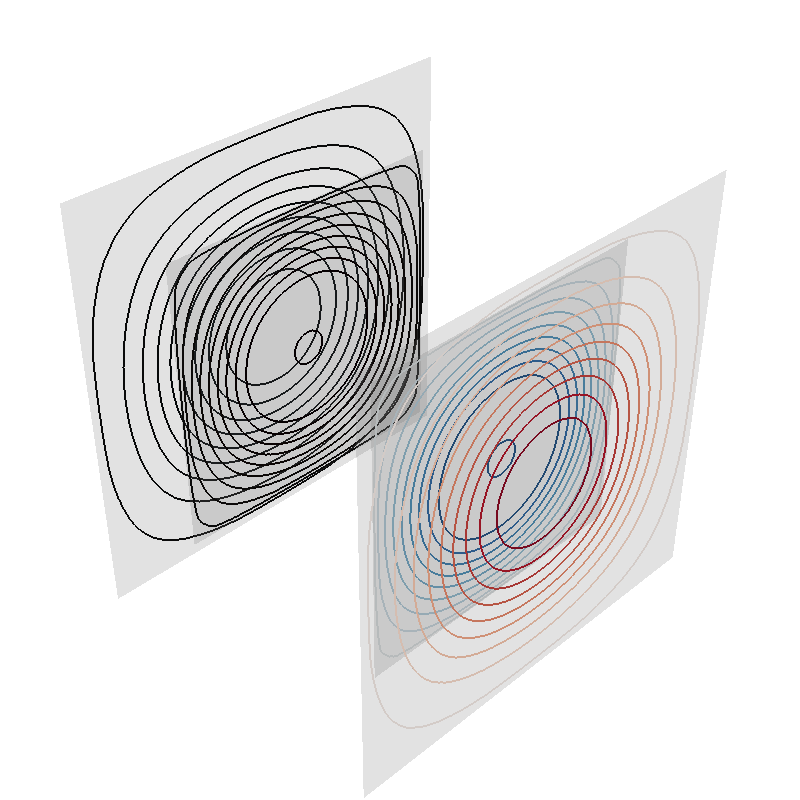
Plot geometry

f = mlab.figure(None, bgcolor=(1, 1, 1), fgcolor=(0.5, 0.5, 0.5), size=(800, 800))
coil.plot_mesh(opacity=0.2, figure=f)
shieldcoil.plot_mesh(opacity=0.2, figure=f)

Out:

<mayavi.core.scene.Scene object at 0x7f0c592711d0>

Compute inductances and coupling

M11 = coil.inductance
M22 = shieldcoil.inductance
M21 = shieldcoil.mutual_inductance(coil)


# Mapping from I1 to I2, constraining flux through shieldcoil to zero
P = -np.linalg.solve(M22, M21)

A1, Beta1 = coil.sph_couplings
A2, Beta2 = shieldcoil.sph_couplings

Out:

Computing the inductance matrix...
Computing self-inductance matrix using rough quadrature (degree=2).              For higher accuracy, set quad_degree to 4 or more.
Estimating 34964 MiB required for 3184 by 3184 vertices...
Computing inductance matrix in 80 chunks (9376 MiB memory free),              when approx_far=True using more chunks is faster...
Computing triangle-coupling matrix
Inductance matrix computation took 13.67 seconds.
Computing the inductance matrix...
Computing self-inductance matrix using rough quadrature (degree=2).              For higher accuracy, set quad_degree to 4 or more.
Estimating 34964 MiB required for 3184 by 3184 vertices...
Computing inductance matrix in 80 chunks (9126 MiB memory free),              when approx_far=True using more chunks is faster...
Computing triangle-coupling matrix
Inductance matrix computation took 13.60 seconds.
Estimating 34964 MiB required for 3184 by 3184 vertices...
Computing inductance matrix in 80 chunks (8985 MiB memory free),              when approx_far=True using more chunks is faster...
Computing triangle-coupling matrix
Computing coupling matrices
l = 1 computed
l = 2 computed
l = 3 computed
l = 4 computed
Computing coupling matrices
l = 1 computed
l = 2 computed
l = 3 computed
l = 4 computed

Precalculations for the solution

# Minimization of magnetic energy with spherical harmonic constraint
C = Beta1 + Beta2 @ P
M = M11 + M21.T @ P

# Regularization
from scipy.linalg import eigvalsh

ssmax = eigvalsh(C.T @ C, M, eigvals=[M.shape[1] - 1, M.shape[1] - 1])

Specify spherical harmonic and calculate corresponding shielded field

beta = np.zeros(Beta1.shape[0])
# beta[7] = 1 # Gradient
beta[2] = 1  # Homogeneous

# Minimum residual
_lambda = 1e3
# Minimum energy
# _lambda=1e-3
I1inner = np.linalg.solve(C.T @ C + M * ssmax / _lambda, C.T @ beta)

I2inner = P @ I1inner

coil.s = StreamFunction(I1inner, coil)
shieldcoil.s = StreamFunction(I2inner, shieldcoil)

Do a quick 3D plot

f = mlab.figure(None, bgcolor=(1, 1, 1), fgcolor=(0.5, 0.5, 0.5), size=(800, 800))

coil.s.plot(figure=f, contours=20)
shieldcoil.s.plot(figure=f, contours=20)

Out:

<mayavi.modules.surface.Surface object at 0x7f0bf986b650>

Compute the field and scalar potential on an XY-plane

x = y = np.linspace(-8, 8, 150)
X, Y = np.meshgrid(x, y, indexing="ij")
points = np.zeros((X.flatten().shape[0], 3))
points[:, 0] = X.flatten()
points[:, 1] = Y.flatten()


CB1 = coil.B_coupling(points)
CB2 = shieldcoil.B_coupling(points)

CU1 = coil.U_coupling(points)
CU2 = shieldcoil.U_coupling(points)

B1 = CB1 @ coil.s
B2 = CB2 @ shieldcoil.s

U1 = CU1 @ coil.s
U2 = CU2 @ shieldcoil.s

Out:

Computing magnetic field coupling matrix, 3184 vertices by 22500 target points... took 15.53 seconds.
Computing magnetic field coupling matrix, 3184 vertices by 22500 target points... took 15.30 seconds.
Computing scalar potential coupling matrix, 3184 vertices by 22500 target points... took 88.08 seconds.
Computing scalar potential coupling matrix, 3184 vertices by 22500 target points... took 94.08 seconds.

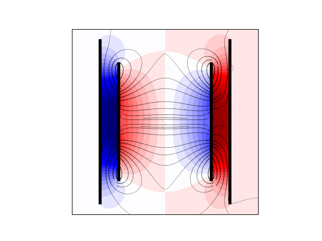
Now, plot the field streamlines and scalar potential

from bfieldtools.contour import scalar_contour

cc1 = scalar_contour(mesh1, mesh1.vertices[:, 2], contours=[-0.001])
cc2 = scalar_contour(mesh2, mesh2.vertices[:, 2], contours=[-0.001])
cx10 = cc1[0][:, 1]
cy10 = cc1[0][:, 0]
cx20 = cc2[0][:, 1]
cy20 = cc2[0][:, 0]

cx11 = np.vstack(cc1[1:])[:, 1]
cy11 = np.vstack(cc1[1:])[:, 0]
cx21 = np.vstack(cc2[1:])[:, 1]
cy21 = np.vstack(cc2[1:])[:, 0]

B = (B1.T + B2.T)[:2].reshape(2, x.shape[0], y.shape[0])
lw = np.sqrt(B[0] ** 2 + B[1] ** 2)
lw = 2 * np.log(lw / np.max(lw) * np.e + 1.1)

xx = np.linspace(-1, 1, 16)

seed_points = np.array([cx10 + 0.001, cy10])
seed_points = np.hstack([seed_points, np.array([cx11 - 0.001, cy11])])
seed_points = np.hstack([seed_points, (0.56 * np.array([np.zeros_like(xx), xx]))])


U = (U1 + U2).reshape(x.shape[0], y.shape[0])
U /= np.max(U)
plt.figure()
plt.contourf(X, Y, U.T, cmap="seismic", levels=40)
# plt.imshow(U, vmin=-1.0, vmax=1.0, cmap='seismic', interpolation='bicubic',
#           extent=(x.min(), x.max(), y.min(), y.max()))
plt.streamplot(
    x,
    y,
    B[1],
    B[0],
    density=2,
    linewidth=lw,
    color="k",
    start_points=seed_points.T,
    integration_direction="both",
    arrowsize=0.1,
)

for loop in cc1 + cc2:
    plt.plot(loop[:, 1], loop[:, 0], "k", linewidth=4, alpha=1)
    plt.plot(-loop[:, 1], -loop[:, 0], "k", linewidth=4, alpha=1)

plt.axis("image")

plt.xticks([])
plt.yticks([])

Out:

([], <a list of 0 Text major ticklabel objects>)

Estimated memory usage: 12747 MB