Interpolate stream function

Minimal example showing how to subdivide a mesh and interpolate a scalar function defined on that mesh to match.

import pyvista as pv
from bfieldtools._example_plots import triangle_mesh, point_cloud

pv.set_plot_theme("document")


import trimesh

import numpy as np
from scipy.linalg import eigh

from bfieldtools.mesh_calculus import laplacian_matrix, mass_matrix
from bfieldtools import utils

from bfieldtools import resources

Load a simple mesh and compute an example scalar function on it. In this case, the scalar function is an eigenvector of a generalized eigenvalue decomposition

mesh = trimesh.load(resources.files("bfieldtools", "example_meshes/10x10_plane.obj"))

boundaries, inner_verts = utils.find_mesh_boundaries(mesh)

L = laplacian_matrix(mesh)
M = mass_matrix(mesh)

u, v = eigh(
    -L.todense()[inner_verts][:, inner_verts], M.todense()[inner_verts][:, inner_verts]
)

scalars = np.zeros(mesh.vertices.shape[0])
scalars[inner_verts] = v[:, 12]


original_scalars = scalars.copy()
original_mesh = mesh.copy()

Plot original scalars and mesh

plotter = scene = pv.Plotter(window_size=(800, 800))

plotter.add_mesh(
    triangle_mesh(*original_mesh.vertices.T, original_mesh.faces),
    scalars=original_scalars,
    style="wireframe",
    show_scalar_bar=False,
)

Static Scene

Interactive Scene

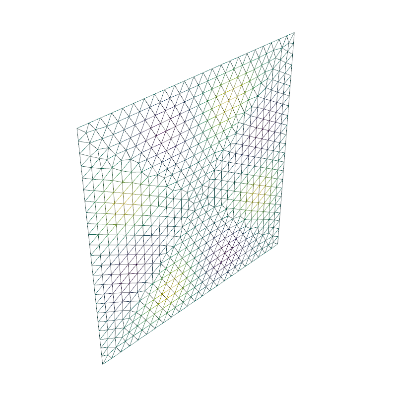
Actor (0x7f12798fb100)
  Center:                     (0.0, 0.0, 0.0)
  Pickable:                   True
  Position:                   (0.0, 0.0, 0.0)
  Scale:                      (1.0, 1.0, 1.0)
  Visible:                    True
  X Bounds                    -5.000E+00, 5.000E+00
  Y Bounds                    0.000E+00, 0.000E+00
  Z Bounds                    -5.000E+00, 5.000E+00
  User matrix:                Identity
  Has mapper:                 True

Property (0x7f12798fafe0)
  Ambient:                     0.0
  Ambient color:               Color(name='light_blue', hex='#add8e6ff', opacity=255)
  Anisotropy:                  0.0
  Color:                       Color(name='light_blue', hex='#add8e6ff', opacity=255)
  Culling:                     "none"
  Diffuse:                     1.0
  Diffuse color:               Color(name='light_blue', hex='#add8e6ff', opacity=255)
  Edge color:                  Color(name='black', hex='#000000ff', opacity=255)
  Edge opacity:                1.0
  Interpolation:               InterpolationType.FLAT
  Lighting:                    True
  Line width:                  1.0
  Metallic:                    0.0
  Opacity:                     1.0
  Point size:                  5.0
  Render lines as tubes:       False
  Render points as spheres:    False
  Roughness:                   0.5
  Show edges:                  False
  Specular:                    0.0
  Specular color:              Color(name='light_blue', hex='#add8e6ff', opacity=255)
  Specular power:              100.0
  Style:                       "Wireframe"

DataSetMapper (0x7f12798fafe0)
  Scalar visibility:           True
  Scalar range:                (-0.2225637118435402, 0.222652285215061)
  Interpolate before mapping:  True
  Scalar map mode:             point
  Color mode:                  map

Attached dataset:
PolyData (0x7f12798fa860)
  N Cells:    1258
  N Points:   676
  N Strips:   0
  X Bounds:   -5.000e+00, 5.000e+00
  Y Bounds:   0.000e+00, 0.000e+00
  Z Bounds:   -5.000e+00, 5.000e+00
  N Arrays:   1

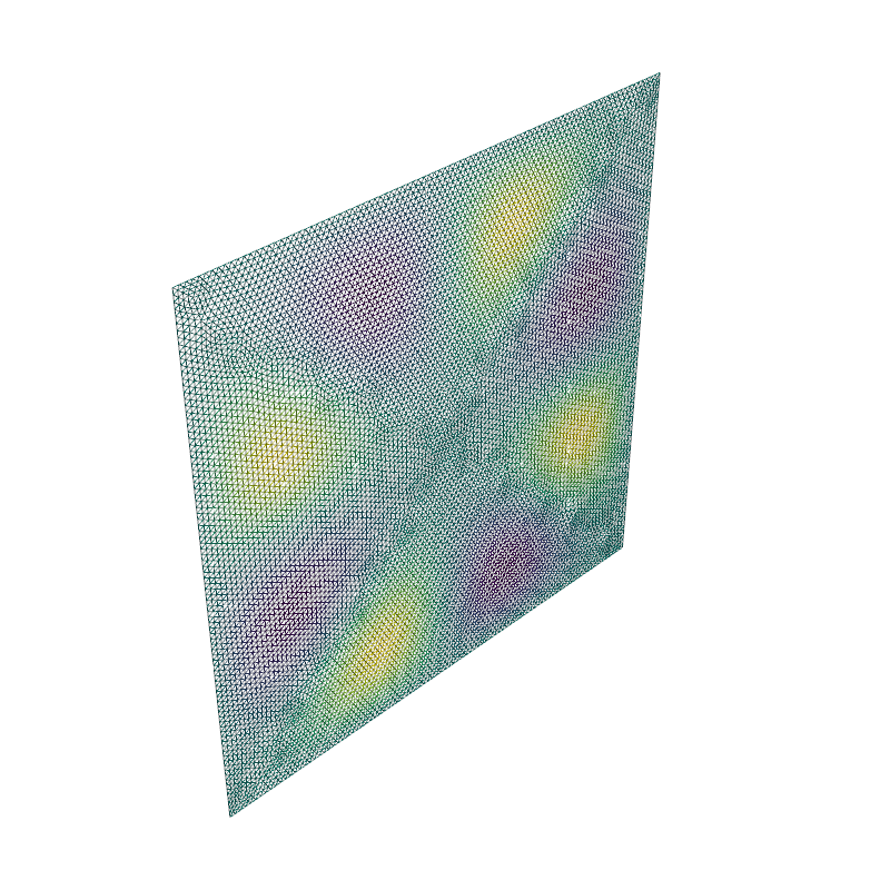
Now, interpolate scalars

ug = triangle_mesh(*mesh.vertices.T, mesh.faces)
ug["scalars"] = scalars


mesh = original_mesh.subdivide().subdivide()
scalars = point_cloud(*mesh.vertices.T).sample(ug)["scalars"]

Plot subdivided mesh and interpolated scalars

plotter = scene = pv.Plotter(window_size=(800, 800))

plotter.add_mesh(
    triangle_mesh(*mesh.vertices.T, mesh.faces),
    scalars=scalars,
    style="wireframe",
    show_scalar_bar=False,
)

# Display the assembled scene (Sphinx-Gallery captures it during docs builds).
if "plotter" in globals() and not plotter._closed:
    plotter.show()

Static Scene

Interactive Scene