Mutual inductance of wire loops

In this example, we demonstrate how to compute the mutual inductance between two sets of polyline wire loops.

from bfieldtools.line_conductor import LineConductor
from bfieldtools.mesh_conductor import StreamFunction
from bfieldtools.suhtools import SuhBasis
from bfieldtools.utils import load_example_mesh

import numpy as np
from mayavi import mlab

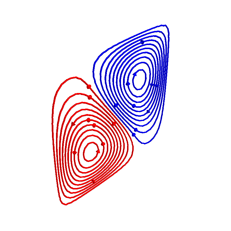
We create a set of wire loops by picking a single (arbitrary) surface-harmonic mode from a plane mesh. Finally, we discretize the mode into a set of wire loops, which we plot.

mesh = load_example_mesh("10x10_plane")
mesh.apply_scale(0.1)  # Downsize from 10 meters to 1 meter
N_contours = 20

sb = SuhBasis(mesh, 10)  # Construct surface-harmonics basis
sf = StreamFunction(
    sb.basis[:, 1], sb.mesh_conductor
)  # Turn single mode into a stream function
c = LineConductor(
    mesh=mesh, scalars=sf, N_contours=N_contours
)  # Discretize the stream function into wire loops


# Plot loops for testing
c.plot_loops(origin=np.array([0, -100, 0]))

Out:

Calculating surface harmonics expansion...
Computing the laplacian matrix...
Computing the mass matrix...

<mayavi.core.scene.Scene object at 0x7fc4fa9fba10>

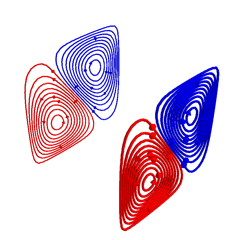
Now, we create a shifted copy of the wire loops, and the calculate the mutual_inductance between two sets of line conductors

mesh2 = mesh.copy()
mesh2.vertices[:, 1] += 1
c2 = LineConductor(mesh=mesh2, scalars=sf, N_contours=N_contours)
fig = c.plot_loops(origin=np.array([0, -100, 0]))
c2.plot_loops(figure=fig, origin=np.array([0, -100, 0]))

Mself = c.line_mutual_inductance(c, separate_loops=True, radius=1e-3)
M2 = c.line_mutual_inductance(c2, separate_loops=True)

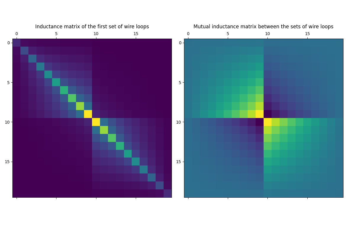
Now, we plot the inductance matrices

import matplotlib.pyplot as plt

ff, ax = plt.subplots(1, 2, figsize=(12, 8))
plt.sca(ax[0])
plt.matshow(Mself, fignum=0)
plt.title("Inductance matrix of the first set of wire loops")
plt.sca(ax[1])
plt.matshow(M2, fignum=0)
plt.title("Mutual inductance matrix between the sets of wire loops")

ff.tight_layout()

The inductance derived from the continous current density

1. Magnetic energy of a inductor is E = 0.5*L*I^2

2. For unit current I=1 the inductance is L=2*E

3. The total current of a stream function (sf) integrated over the from minimum to maximum is dsf = max(sf) - min(sf)

4. When discretized to N conductors the current per conductor is I = dsf / N

5. When sf is normalized such that I=1, i.e., dsf = N the inductance approximated by the continous stream function is L = 2*sf.magnetic_energy

scaling = N_contours / (sf.max() - sf.min())
L_approx = 2 * sf.magnetic_energy * (scaling ** 2)

print("Inductance based on the continuous current density", L_approx)
print("Inductance based on r=1mm wire", np.sum(Mself))

Out:

Computing the inductance matrix...
Computing self-inductance matrix using rough quadrature (degree=2).              For higher accuracy, set quad_degree to 4 or more.
Estimating 2432 MiB required for 676 by 676 vertices...
Computing inductance matrix in 20 chunks (3990 MiB memory free),              when approx_far=True using more chunks is faster...
Computing triangle-coupling matrix
Inductance matrix computation took 1.31 seconds.
Inductance based on the continuous current density 8.689344781849715e-05
Inductance based on r=1mm wire 9.793656583088348e-05

Estimated memory usage: 133 MB