Field of a Helmholtz coils pair

Example on how to compute the magnetic field from current line segments forming a Helmholtz coil pair.

Visualization of the 3D field using Mayavi

from mayavi import mlab
import matplotlib.pyplot as plt
import numpy as np

from bfieldtools.utils import cylinder_points
from bfieldtools.line_magnetics import magnetic_field

# Create helmholtz coil with radius R
R = 5

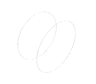
c_points = cylinder_points(
    radius=R, length=0, nlength=1, nalpha=100, orientation=np.array([0, 1, 0])
)
c_points[:, 1] = 0
c_points = np.vstack((c_points, c_points[0, :]))


c1_points = c_points - np.array([0, R / 2, 0])
c2_points = c_points + np.array([0, R / 2, 0])

mlab.figure(bgcolor=(1, 1, 1))
mlab.plot3d(*c1_points.T)
mlab.plot3d(*c2_points.T)

box = 3 * R
n = 50

xx = np.linspace(-box, box, n)
yy = np.linspace(-box, box, n)
zz = np.linspace(-box, box, n)
X, Y, Z = np.meshgrid(xx, yy, zz, indexing="ij")

x = X.ravel()
y = Y.ravel()
z = Z.ravel()

b_points = np.array([x, y, z]).T

B = np.zeros(b_points.shape)

B += magnetic_field(c1_points, b_points)
B += magnetic_field(c2_points, b_points)


B_matrix = B.reshape((n, n, n, 3))

B_matrix_norm = np.linalg.norm(B_matrix, axis=-1)

mlab.figure(bgcolor=(1, 1, 1))

field = mlab.pipeline.vector_field(
    X,
    Y,
    Z,
    B_matrix[:, :, :, 0],
    B_matrix[:, :, :, 1],
    B_matrix[:, :, :, 2],
    scalars=B_matrix_norm,
    name="B-field",
)

vectors = mlab.pipeline.vectors(field, scale_factor=(X[1, 0, 0] - X[0, 0, 0]),)


vectors.glyph.mask_input_points = True
vectors.glyph.mask_points.on_ratio = 2

vcp = mlab.pipeline.vector_cut_plane(field)
vcp.glyph.glyph.scale_factor = 10 * (X[1, 0, 0] - X[0, 0, 0])
# For prettier picture:
vcp.implicit_plane.widget.enabled = True

iso = mlab.pipeline.iso_surface(field, contours=10, opacity=0.2, colormap="viridis")


# A trick to make transparency look better: cull the front face
iso.actor.property.frontface_culling = True

# Settings
iso.contour.maximum_contour = 1e-07
vcp.implicit_plane.widget.normal_to_y_axis = True

plt.figure()

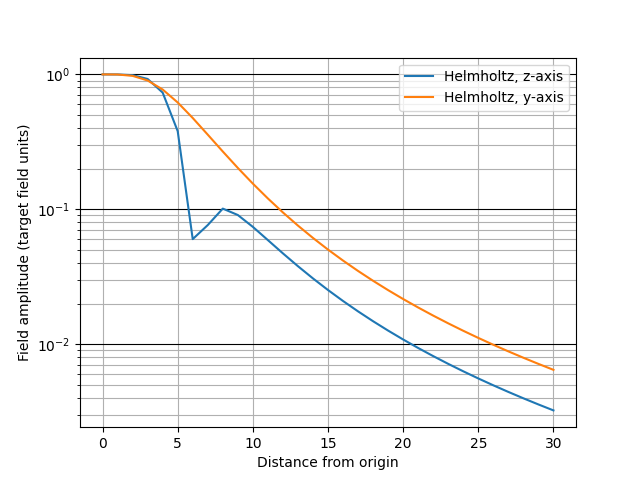
z1 = np.linspace(0, 30, 31)

x1 = y1 = np.zeros_like(z1)

line1_points = np.vstack((x1, y1, z1)).T


Bh_line1 = magnetic_field(c1_points, line1_points) + magnetic_field(
    c2_points, line1_points
)

plt.semilogy(
    z1,
    np.linalg.norm(Bh_line1, axis=1) / np.linalg.norm(Bh_line1, axis=1)[0],
    label="Helmholtz, z-axis",
)


y2 = np.linspace(0, 30, 31)

z2 = x2 = np.zeros_like(y2)

line2_points = np.vstack((x2, y2, z2)).T

Bh_line2 = magnetic_field(c1_points, line2_points) + magnetic_field(
    c2_points, line2_points
)


plt.semilogy(
    y2,
    np.linalg.norm(Bh_line2, axis=1) / np.linalg.norm(Bh_line2, axis=1)[0],
    label="Helmholtz, y-axis",
)
plt.ylabel("Field amplitude (target field units)")
plt.xlabel("Distance from origin")
plt.grid(True, which="minor", axis="y")
plt.grid(True, which="major", axis="y", color="k")
plt.grid(True, which="major", axis="x")

plt.legend()

Out:

<matplotlib.legend.Legend object at 0x7fc4c85c6650>

Estimated memory usage: 65 MB