Note
Click here to download the full example code
Biplanar coil design
First example in the paper, showing a basic biplanar coil producing homogeneous field in a target region between the two coil planes.
PLOT = True
SAVE_FIGURES = False

SAVE_DIR = "./Biplanar coil/"


import numpy as np
from mayavi import mlab
import trimesh

from bfieldtools.mesh_conductor import MeshConductor
from bfieldtools.coil_optimize import optimize_streamfunctions
from bfieldtools.contour import scalar_contour
from bfieldtools.viz import plot_3d_current_loops
from bfieldtools.utils import load_example_mesh, combine_meshes


# Set unit, e.g. meter or millimeter.
# This doesn't matter, the problem is scale-invariant
scaling_factor = 1


# Load simple plane mesh that is centered on the origin
planemesh = load_example_mesh("10x10_plane_hires")


# Specify coil plane geometry
center_offset = np.array([0, 0, 0]) * scaling_factor
standoff = np.array([0, 5, 0]) * scaling_factor

# Create coil plane pairs
coil_plus = trimesh.Trimesh(
    planemesh.vertices + center_offset + standoff, planemesh.faces, process=False
)

coil_minus = trimesh.Trimesh(
    planemesh.vertices + center_offset - standoff, planemesh.faces, process=False
)

joined_planes = combine_meshes((coil_plus, coil_minus))

joined_planes = joined_planes.subdivide()

# Create mesh class object
coil = MeshConductor(
    verts=joined_planes.vertices,
    tris=joined_planes.faces,
    fix_normals=True,
    basis_name="suh",
    N_suh=100,
)
Out:
Calculating surface harmonics expansion...
Computing the laplacian matrix...
Computing the mass matrix...
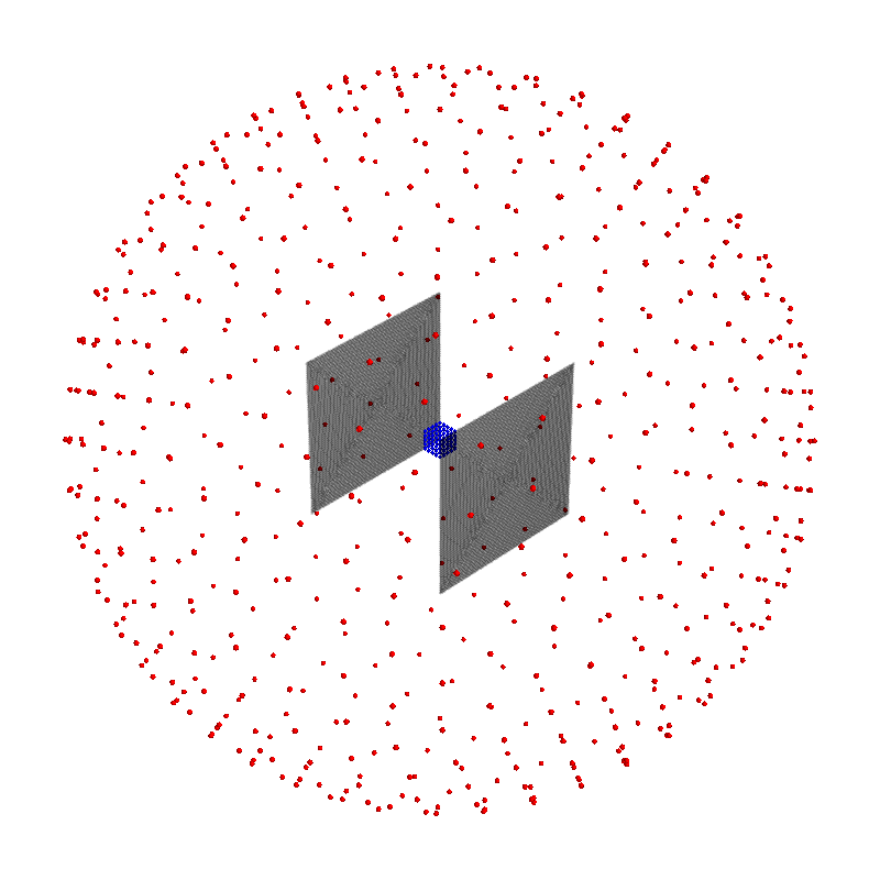
Set up target and stray field points
# Here, the target points are on a volumetric grid within a sphere

center = np.array([0, 0, 0]) * scaling_factor

sidelength = 2 * scaling_factor
n = 8
xx = np.linspace(-sidelength / 2, sidelength / 2, n)
yy = np.linspace(-sidelength / 2, sidelength / 2, n)
zz = np.linspace(-sidelength / 2, sidelength / 2, n)
X, Y, Z = np.meshgrid(xx, yy, zz, indexing="ij")

x = X.ravel()
y = Y.ravel()
z = Z.ravel()

target_points = np.array([x, y, z]).T

# Turn cube into sphere by rejecting points "in the corners"
target_points = (
    target_points[np.linalg.norm(target_points, axis=1) < sidelength / 2] + center
)


#    #Here, the stray field points are on a spherical surface
stray_radius = 20 * scaling_factor

stray_points_mesh = trimesh.creation.icosphere(subdivisions=3, radius=stray_radius)
stray_points = stray_points_mesh.vertices + center

n_stray_points = len(stray_points)
Plot geometry
if PLOT:
    f = mlab.figure(None, bgcolor=(1, 1, 1), fgcolor=(0.5, 0.5, 0.5), size=(800, 800))

    coil.plot_mesh(representation="wireframe", opacity=0.1, color=(0, 0, 0), figure=f)
    coil.plot_mesh(representation="surface", opacity=0.1, color=(0, 0, 0), figure=f)
    mlab.points3d(*target_points.T, color=(0, 0, 1))
    mlab.points3d(*stray_points.T, scale_factor=0.3, color=(1, 0, 0))

    f.scene.isometric_view()
    f.scene.camera.zoom(1.5)

    if SAVE_FIGURES:
        mlab.savefig(
            SAVE_DIR + "biplanar_geometry.png", figure=f, magnification=4,
        )
        mlab.close()
Create bfield specifications used when optimizing the coil geometry
# The absolute target field amplitude is not of importance,
# and it is scaled to match the C matrix in the optimization function

target_field = np.zeros(target_points.shape)
target_field[:, 0] += 1  # Homogeneous field on X-axis


target_spec = {
    "coupling": coil.B_coupling(target_points),
    "abs_error": 0.005,
    "target": target_field,
}
stray_spec = {
    "coupling": coil.B_coupling(stray_points),
    "abs_error": 0.01,
    "target": np.zeros((n_stray_points, 3)),
}

bfield_specification = [target_spec, stray_spec]
Out:
Computing magnetic field coupling matrix, 12442 vertices by 160 target points... took 1.03 seconds.
Computing magnetic field coupling matrix, 12442 vertices by 642 target points... took 2.40 seconds.
Run QP solver
import mosek

coil.s, prob = optimize_streamfunctions(
    coil,
    [target_spec, stray_spec],
    objective=(0, 1),
    solver="MOSEK",
    solver_opts={"mosek_params": {mosek.iparam.num_threads: 8}},
)
Out:
Computing the resistance matrix...
Passing problem to solver...


Problem
  Name                   :
  Objective sense        : min
  Type                   : CONIC (conic optimization problem)
  Constraints            : 4914
  Cones                  : 1
  Scalar variables       : 203
  Matrix variables       : 0
  Integer variables      : 0

Optimizer started.
Problem
  Name                   :
  Objective sense        : min
  Type                   : CONIC (conic optimization problem)
  Constraints            : 4914
  Cones                  : 1
  Scalar variables       : 203
  Matrix variables       : 0
  Integer variables      : 0

Optimizer  - threads                : 8
Optimizer  - solved problem         : the dual
Optimizer  - Constraints            : 101
Optimizer  - Cones                  : 1
Optimizer  - Scalar variables       : 4914              conic                  : 102
Optimizer  - Semi-definite variables: 0                 scalarized             : 0
Factor     - setup time             : 0.02              dense det. time        : 0.00
Factor     - ML order time          : 0.00              GP order time          : 0.00
Factor     - nonzeros before factor : 5151              after factor           : 5151
Factor     - dense dim.             : 0                 flops                  : 2.43e+07
ITE PFEAS    DFEAS    GFEAS    PRSTATUS   POBJ              DOBJ              MU       TIME
0   8.2e+01  1.0e+00  2.0e+00  0.00e+00   0.000000000e+00   -1.000000000e+00  1.0e+00  0.13
1   6.0e+01  7.3e-01  1.6e+00  -9.04e-01  3.692543712e-01   -3.050100236e-01  7.3e-01  0.14
2   3.9e+01  4.7e-01  1.2e+00  -7.84e-01  3.882618770e+00   3.711566228e+00   4.7e-01  0.15
3   3.5e+01  4.2e-01  1.1e+00  -5.93e-01  6.287459499e+00   6.223391554e+00   4.2e-01  0.15
4   2.6e+01  3.2e-01  8.5e-01  -5.39e-01  2.034139252e+01   2.054920828e+01   3.2e-01  0.16
5   1.6e+01  2.0e-01  5.5e-01  -4.07e-01  2.816131282e+01   2.876137058e+01   2.0e-01  0.17
6   1.3e+01  1.5e-01  4.2e-01  -1.88e-01  1.768069636e+02   1.774783265e+02   1.5e-01  0.17
7   6.3e+00  7.7e-02  2.0e-01  -5.34e-02  2.542809795e+02   2.551307604e+02   7.7e-02  0.18
8   4.5e+00  5.5e-02  1.3e-01  2.39e-01   5.348575124e+02   5.356788432e+02   5.5e-02  0.18
9   1.1e+00  1.3e-02  2.2e-02  3.52e-01   1.758584167e+03   1.759055080e+03   1.3e-02  0.19
10  3.4e-01  4.2e-03  4.2e-03  8.21e-01   2.335518573e+03   2.335698877e+03   4.2e-03  0.20
11  2.5e-01  3.0e-03  3.5e-03  7.76e-01   2.357020802e+03   2.357279805e+03   3.0e-03  0.21
12  1.1e-01  1.3e-03  2.0e-03  -1.72e-01  2.605656909e+03   2.606141160e+03   1.3e-03  0.21
13  3.6e-02  4.4e-04  9.1e-04  -4.95e-01  3.624825070e+03   3.625847689e+03   4.4e-04  0.22
14  1.9e-02  2.3e-04  4.4e-04  -1.47e-01  5.980498055e+03   5.981376113e+03   2.3e-04  0.23
15  8.9e-03  1.1e-04  2.8e-04  -4.45e-01  7.027383841e+03   7.029059070e+03   1.1e-04  0.23
16  3.8e-03  4.6e-05  7.1e-05  5.67e-01   1.213232522e+04   1.213289653e+04   4.6e-05  0.24
17  4.1e-04  4.9e-06  2.7e-06  6.25e-01   1.579455105e+04   1.579462556e+04   4.9e-06  0.25
18  1.1e-05  1.3e-07  1.8e-08  9.57e-01   1.636071777e+04   1.636072230e+04   1.3e-07  0.26
19  1.5e-06  1.9e-08  1.0e-09  9.98e-01   1.637943536e+04   1.637943604e+04   1.9e-08  0.27
20  1.2e-07  7.3e-11  1.4e-11  1.00e+00   1.638250423e+04   1.638250423e+04   7.3e-11  0.30
21  9.2e-08  7.3e-11  3.4e-12  1.00e+00   1.638250424e+04   1.638250424e+04   7.3e-11  0.32
22  9.2e-08  7.3e-11  3.4e-12  1.00e+00   1.638250424e+04   1.638250424e+04   7.3e-11  0.34
23  9.2e-08  7.3e-11  3.4e-12  1.00e+00   1.638250424e+04   1.638250424e+04   7.3e-11  0.37
24  1.6e-07  6.6e-11  1.4e-12  1.00e+00   1.638250541e+04   1.638250541e+04   6.6e-11  0.39
25  1.8e-07  6.4e-11  2.1e-12  1.00e+00   1.638250568e+04   1.638250568e+04   6.4e-11  0.41
26  2.0e-07  6.4e-11  6.5e-12  1.00e+00   1.638250570e+04   1.638250570e+04   6.4e-11  0.44
27  2.0e-07  6.4e-11  2.6e-12  1.00e+00   1.638250573e+04   1.638250573e+04   6.4e-11  0.46
28  2.5e-07  5.8e-11  3.4e-12  1.00e+00   1.638250679e+04   1.638250679e+04   5.8e-11  0.48
29  2.4e-07  5.8e-11  2.4e-12  1.00e+00   1.638250680e+04   1.638250680e+04   5.7e-11  0.50
30  4.8e-07  3.4e-11  4.4e-13  1.00e+00   1.638251067e+04   1.638251068e+04   3.4e-11  0.52
Optimizer terminated. Time: 0.53


Interior-point solution summary
  Problem status  : PRIMAL_AND_DUAL_FEASIBLE
  Solution status : OPTIMAL
  Primal.  obj: 1.6382510674e+04    nrm: 3e+04    Viol.  con: 7e-09    var: 0e+00    cones: 0e+00
  Dual.    obj: 1.6382510676e+04    nrm: 6e+05    Viol.  con: 0e+00    var: 1e-09    cones: 0e+00
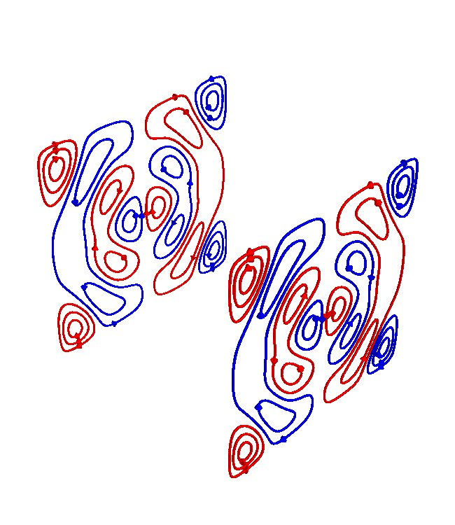
Plot coil windings and target points
N_contours = 6

loops = scalar_contour(coil.mesh, coil.s.vert, N_contours=N_contours)

if PLOT:
    f = mlab.figure(None, bgcolor=(1, 1, 1), fgcolor=(0.5, 0.5, 0.5), size=(650, 750))
    mlab.clf()

    plot_3d_current_loops(loops, colors="auto", figure=f)

    # B_target = coil.B_coupling(target_points) @ coil.s

    # mlab.quiver3d(*target_points.T, *B_target.T, mode="arrow", scale_factor=1)

    f.scene.isometric_view()
    #    f.scene.camera.zoom(0.95)
    if SAVE_FIGURES:
        mlab.savefig(
            SAVE_DIR + "biplanar_loops.png", figure=f, magnification=4,
        )

        mlab.close()
Plot continuous stream function
if PLOT:
    from bfieldtools.viz import plot_data_on_vertices

    f = mlab.figure(None, bgcolor=(1, 1, 1), fgcolor=(0.5, 0.5, 0.5), size=(800, 800))
    mlab.clf()

    plot_data_on_vertices(coil.mesh, coil.s.vert, figure=f, ncolors=256)

    f.scene.camera.parallel_projection = 1
    mlab.view(90, 90)
    f.scene.camera.zoom(1.5)

    if SAVE_FIGURES:
        mlab.savefig(
            SAVE_DIR + "biplanar_streamfunction.png", figure=f, magnification=4,
        )

        mlab.close()

Total running time of the script: ( 0 minutes 15.762 seconds)
Estimated memory usage: 1586 MB