SUH-SPH interpolation comparison

import numpy as np
from bfieldtools.mesh_conductor import MeshConductor, StreamFunction
from mayavi import mlab
import trimesh
import matplotlib.pyplot as plt

from bfieldtools.sphtools import basis_fields as sphfield
from bfieldtools.sphtools import field as sph_field_eval
from bfieldtools.sphtools import basis_potentials, potential
import mne

from bfieldtools.viz import plot_data_on_vertices, plot_mesh

SAVE_DIR = "./MNE interpolation/"

EVOKED = True

with np.load(SAVE_DIR + "mne_data.npz", allow_pickle=True) as data:
    p = data["p"]
    n = data["n"]
    mesh = trimesh.Trimesh(vertices=data["vertices"], faces=data["faces"])

if EVOKED:
    evoked = mne.Evoked(SAVE_DIR + "left_auditory-ave.fif")

    i0, i1 = evoked.time_as_index(0.08)[0], evoked.time_as_index(0.09)[0]
    field = evoked.data[:, i0:i1].mean(axis=1)

else:
    # take "data" from lead field matrix, i.e, topography of a single dipole
    from mne.datasets import sample
    import os

    data_path = sample.data_path()

    raw_fname = data_path + "/MEG/sample/sample_audvis_raw.fif"
    trans = data_path + "/MEG/sample/sample_audvis_raw-trans.fif"
    src = data_path + "/subjects/sample/bem/sample-oct-6-src.fif"
    bem = data_path + "/subjects/sample/bem/sample-5120-5120-5120-bem-sol.fif"
    subjects_dir = os.path.join(data_path, "subjects")

    # Note that forward solutions can also be read with read_forward_solution
    fwd = mne.make_forward_solution(
        raw_fname, trans, src, bem, meg=True, eeg=False, mindist=5.0, n_jobs=2
    )
    # Take only magnetometers
    mags = np.array([n[-1] == "1" for n in fwd["sol"]["row_names"]])
    L = fwd["sol"]["data"][mags, :]
    # Take the first dipole
    field = L[:, 56]

Out:

    Read a total of 4 projection items:
        PCA-v1 (1 x 102) active
        PCA-v2 (1 x 102) active
        PCA-v3 (1 x 102) active
        Average EEG reference (1 x 60) active
    Found the data of interest:
        t =    -199.80 ...     499.49 ms (Left Auditory)
        0 CTF compensation matrices available
        nave = 55 - aspect type = 100
Projections have already been applied. Setting proj attribute to True.

R = np.min(np.linalg.norm(p, axis=1)) - 0.02

lmax = 7  # maximum degree
Bca, Bcb = sphfield(p, lmax, normalization="energy", R=R)

# sph-components at sensors
Bca_sensors = np.einsum("ijk,ij->ik", Bca, n)
Bcb_sensors = np.einsum("ijk,ij->ik", Bcb, n)

idx = 20

# evoked1 = evoked.copy()
# evoked1.data[:, :] = np.tile(Bca_sensors[:, idx].T, (evoked.times.shape[0], 1)).T
# evoked1.plot_topomap(times=0.080, ch_type="mag", colorbar=False)

# evoked1 = evoked.copy()
# evoked1.data[:, :] = np.tile(Bcb_sensors[:, idx].T, (evoked.times.shape[0], 1)).T
# evoked1.plot_topomap(times=0.080, ch_type="mag", colorbar=False)

PINV = True
if PINV:
    alpha = np.linalg.pinv(Bca_sensors, rcond=1e-15) @ field
else:
    # Calculate using regularization
    ssa = np.linalg.svd(Bca_sensors @ Bca_sensors.T, False, False)
    reg_exp = 6
    _lambda = np.max(ssa) * (10 ** (-reg_exp))
    # angular-Laplacian in the sph basis is diagonal
    La = np.diag([l * (l + 1) for l in range(1, lmax + 1) for m in range(-l, l + 1)])
    BB = Bca_sensors.T @ Bca_sensors + _lambda * La
    alpha = np.linalg.solve(BB, Bca_sensors.T @ field)

# Reconstruct field in helmet

# reco_sph = np.zeros(field.shape)
# i = 0
# for l in range(1, lmax + 1):
#     for m in range(-1 * l, l + 1):
#         reco_sph += alpha[i] * Bca_sensors[:, i]
#         i += 1

# Produces the same result as the loop
reco_sph = Bca_sensors @ alpha

print(
    "SPH-reconstruction relative error:",
    np.linalg.norm(reco_sph - field) / np.linalg.norm(field),
)

Out:

SPH-reconstruction relative error: 0.03031555824094214

#%% Fit the surface current for the auditory evoked response using pinv

c = MeshConductor(mesh_obj=mesh, basis_name=”suh”, N_suh=35) M = c.mass B_sensors = np.einsum(“ijk,ij->ik”, c.B_coupling(p), n)

asuh = np.linalg.pinv(B_sensors, rcond=1e-15) @ field

s = StreamFunction(asuh, c) b_filt = B_sensors @ s

c = MeshConductor(mesh_obj=mesh, basis_name="suh", N_suh=150)
M = c.mass

B_sensors = np.einsum("ijk,ij->ik", c.B_coupling(p), n)
ss = np.linalg.svd(B_sensors @ B_sensors.T, False, False)

reg_exp = 1
plot_this = True
rel_errors = []
_lambda = np.max(ss) * (10 ** (-reg_exp))
# Laplacian in the suh basis is diagonal
BB = B_sensors.T @ B_sensors + _lambda * (-c.laplacian) / np.max(abs(c.laplacian))
a = np.linalg.solve(BB, B_sensors.T @ field)

s = StreamFunction(a, c)

reco_suh = B_sensors @ s

print(
    "SUH-reconstruction relative error:",
    np.linalg.norm(reco_suh - field) / np.linalg.norm(field),
)

f = mlab.figure(bgcolor=(1, 1, 1))
surf = s.plot(False, figure=f)
surf.actor.mapper.interpolate_scalars_before_mapping = True
surf.module_manager.scalar_lut_manager.number_of_colors = 16

Out:

Calculating surface harmonics expansion...
Computing the laplacian matrix...
Computing the mass matrix...
Closed mesh or Neumann BC, leaving out the constant component
Computing the mass matrix...
Computing magnetic field coupling matrix, 2562 vertices by 102 target points... took 0.19 seconds.
Computing the laplacian matrix...
SUH-reconstruction relative error: 0.020549237736974476

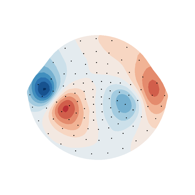
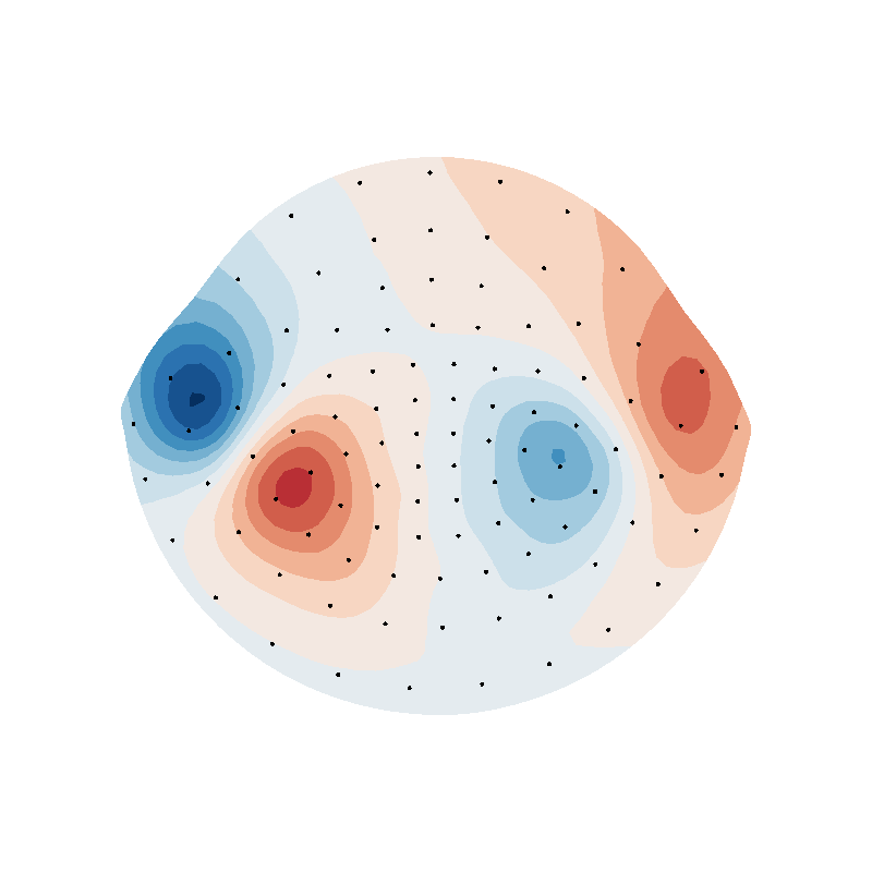
evoked1 = evoked.copy() evoked1.data[:, :] = np.tile(field.T, (evoked.times.shape[0], 1)).T evoked1.plot_topomap(times=0.080, ch_type=”mag”)

# evoked1 = evoked.copy()
# evoked1.data[:, :] = np.tile(reco_sph.T, (evoked.times.shape[0], 1)).T
# evoked1.plot_topomap(times=0.080, ch_type="mag")


# evoked1 = evoked.copy()
# evoked1.data[:, :] = np.tile(reco_suh.T, (evoked.times.shape[0], 1)).T
# evoked1.plot_topomap(times=0.080, ch_type="mag")

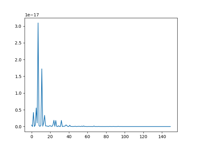
fig, ax = plt.subplots(1, 1)
ax.plot(alpha ** 2)


L = np.zeros((0,))
M = np.zeros((0,))


for l in range(1, lmax + 1):
    m_l = np.arange(-l, l + 1, step=1, dtype=np.int_)
    M = np.append(M, m_l)
    L = np.append(L, np.repeat(l, len(m_l)))

xticknames = [None] * len(alpha)
for i in range(len(alpha)):
    xticknames[i] = str(M[i])

    m_l = np.arange(-L[i], L[i] + 1, step=1)

    if i == int(np.floor(len(m_l))):
        xticknames[i] += "\n" + str(L[i])


plt.figure()
plt.plot(a ** 2)

• 
• 

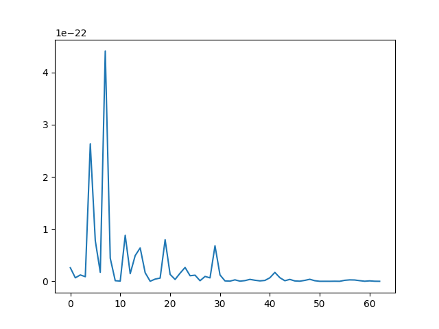
Out:

[<matplotlib.lines.Line2D object at 0x7f94d943d190>]

from bfieldtools.utils import load_example_mesh
from bfieldtools.flatten_mesh import flatten_mesh, mesh2plane

helmet = load_example_mesh("meg_helmet", process=False)
# Bring the surface roughly to the correct place
helmet.vertices[:, 2] -= 0.045
# The helmet is slightly tilted, correct for this
# (probably the right coordinate transformation could be found from MNE)
rotmat = np.eye(3)
tt = 0.015 * np.pi
rotmat[:2, :2] = np.array([[np.cos(tt), np.sin(tt)], [-np.sin(tt), np.cos(tt)]])
helmet.vertices = helmet.vertices @ rotmat
tt = -0.02 * np.pi
rotmat[1:, 1:] = np.array([[np.cos(tt), np.sin(tt)], [-np.sin(tt), np.cos(tt)]])
helmet.vertices = helmet.vertices @ rotmat
helmet.vertices[:, 1] += 0.005

# plot_mesh(helmet)
# mlab.points3d(*p.T, scale_factor=0.01)


B_sph_helmet = sph_field_eval(
    helmet.vertices,
    alpha,
    np.zeros(alpha.shape),
    lmax=lmax,
    normalization="energy",
    R=R,
)
B_sph_helmet = np.einsum("ij,ij->i", B_sph_helmet, helmet.vertex_normals)
B_suh_helmet = c.B_coupling(helmet.vertices) @ s
B_suh_helmet = np.einsum("ij,ij->i", B_suh_helmet, helmet.vertex_normals)

Out:

Computing magnetic field coupling matrix, 2562 vertices by 2044 target points... took 1.64 seconds.

u, v, helmet2d = flatten_mesh(helmet, 0.9)
puv = mesh2plane(p, helmet, u, v)

Out:

[[4.77790946e-01 4.66308115e-01 5.59009381e-02]
 [5.04848824e-01 4.42294362e-01 5.28568138e-02]
 [4.15888839e-01 2.50513180e-01 3.33597981e-01]
 [2.06948013e-01 5.88223293e-01 2.04828694e-01]
 [7.43679193e-01 1.41597623e-02 2.42161044e-01]
 [2.60921217e-01 1.20738365e-01 6.18340418e-01]
 [1.06206809e-01 4.65233540e-01 4.28559651e-01]
 [4.23861276e-01 2.85462097e-01 2.90676627e-01]
 [4.62148412e-01 4.52560953e-01 8.52906351e-02]
 [3.09306223e-02 8.52708268e-01 1.16361110e-01]
 [2.70379534e-01 6.81687446e-01 4.79330195e-02]
 [4.59313482e-01 3.12962219e-01 2.27724300e-01]
 [6.92782782e-01 4.97428360e-02 2.57474382e-01]
 [1.29101813e-01 1.64312903e-01 7.06585284e-01]
 [3.36234522e-01 2.74311949e-01 3.89453530e-01]
 [4.13475354e-01 3.73633628e-01 2.12891018e-01]
 [8.33417794e-01 1.57603804e-01 8.97840261e-03]
 [7.98616179e-01 9.00989335e-02 1.11284888e-01]
 [8.03083739e-01 6.64707125e-02 1.30445549e-01]
 [4.20927343e-01 4.28587408e-01 1.50485249e-01]
 [8.18570681e-01 4.51420621e-02 1.36287257e-01]
 [1.15661059e-01 5.62169746e-01 3.22169194e-01]
 [2.47303261e-01 4.95183716e-01 2.57513024e-01]
 [3.84895035e-01 4.70099315e-01 1.45005650e-01]
 [1.88017253e-01 7.40471379e-01 7.15113683e-02]
 [6.74873443e-01 9.61318319e-02 2.28994725e-01]
 [1.59982479e-01 8.11252699e-01 2.87648212e-02]
 [4.64517071e-01 4.27399733e-01 1.08083197e-01]
 [7.54474593e-02 5.85757656e-01 3.38794884e-01]
 [1.08843711e-01 8.13037122e-01 7.81191668e-02]
 [3.43369501e-01 3.13493214e-01 3.43137284e-01]
 [1.85170017e-01 2.30579710e-01 5.84250273e-01]
 [6.79646872e-01 2.67706147e-01 5.26469810e-02]
 [1.89212972e-02 8.60663857e-01 1.20414846e-01]
 [2.19693188e-01 2.64810472e-01 5.15496340e-01]
 [7.98823957e-02 9.34769612e-02 8.26640643e-01]
 [7.14094442e-02 8.31475458e-01 9.71150982e-02]
 [2.59097013e-01 1.68490975e-01 5.72412012e-01]
 [4.07343600e-01 5.11036819e-01 8.16195811e-02]
 [1.32717971e-01 8.33138582e-01 3.41434471e-02]
 [3.13462614e-01 1.48062662e-01 5.38474724e-01]
 [7.42881759e-01 3.12088539e-03 2.53997356e-01]
 [2.96876194e-01 4.98077092e-01 2.05046714e-01]
 [3.65814138e-01 2.62254712e-01 3.71931150e-01]
 [1.10720060e-02 8.64955708e-01 1.23972286e-01]
 [3.21144032e-01 4.86537021e-01 1.92318946e-01]
 [1.04443169e-01 5.71941118e-01 3.23615713e-01]
 [4.50790738e-01 2.19189994e-01 3.30019268e-01]
 [4.04778105e-01 4.00887623e-01 1.94334273e-01]
 [3.18676147e-01 1.28560681e-01 5.52763172e-01]
 [2.76242426e-01 1.41158119e-01 5.82599454e-01]
 [6.37868960e-01 1.95355662e-01 1.66775377e-01]
 [5.50284086e-01 1.22559125e-01 3.27156789e-01]
 [3.91686577e-01 3.21600278e-01 2.86713144e-01]
 [6.41682583e-01 1.75384412e-02 3.40778975e-01]
 [3.74331903e-01 6.11714862e-01 1.39532357e-02]
 [4.91429595e-01 2.63888562e-01 2.44681844e-01]
 [6.35704510e-01 4.43918667e-02 3.19903623e-01]
 [4.61609699e-01 4.64453618e-01 7.39366822e-02]
 [2.29987050e-01 6.06818740e-01 1.63194210e-01]
 [4.49050475e-01 5.19773901e-02 4.98972135e-01]
 [1.78305352e-01 8.02680348e-01 1.90143004e-02]
 [5.92190154e-01 2.36098014e-01 1.71711832e-01]
 [5.32022306e-01 6.23686733e-02 4.05609021e-01]
 [8.45463806e-01 1.41576509e-01 1.29596841e-02]
 [2.72054347e-01 6.96928499e-01 3.10171545e-02]
 [1.64155952e-01 4.80567404e-01 3.55276644e-01]
 [3.01494502e-02 8.05901183e-01 1.63949366e-01]
 [8.07603124e-01 5.70982717e-02 1.35298604e-01]
 [5.12699459e-02 8.48197335e-01 1.00532719e-01]
 [9.92918764e-02 8.13559843e-01 8.71482810e-02]
 [2.95361027e-02 8.54295204e-01 1.16168693e-01]
 [1.52681899e-01 1.70938516e-01 6.76379585e-01]
 [5.22745635e-01 2.39884144e-02 4.53265951e-01]
 [3.05745434e-01 6.45469198e-01 4.87853678e-02]
 [2.49609614e-01 5.60223186e-01 1.90167200e-01]
 [2.49872837e-01 4.36461163e-01 3.13665999e-01]
 [1.64160685e-01 6.01108400e-01 2.34730915e-01]
 [1.26418576e-01 7.73225941e-01 1.00355483e-01]
 [3.63806414e-01 8.45752805e-02 5.51618306e-01]
 [3.12551064e-01 3.64475961e-01 3.22972975e-01]
 [2.32512251e-01 3.00794031e-01 4.66693718e-01]
 [3.67268508e-01 4.18395990e-01 2.14335502e-01]
 [6.60337685e-01 9.38646701e-02 2.45797645e-01]
 [2.55563841e-01 7.04043603e-01 4.03925562e-02]
 [1.01576353e-01 9.44391259e-02 8.03984521e-01]
 [8.30444738e-01 1.69555262e-01 3.19874442e-16]
 [5.94903548e-02 4.95979689e-01 4.44529956e-01]
 [4.72055368e-01 4.90818032e-01 3.71265995e-02]
 [5.13788461e-02 2.92824093e-01 6.55797060e-01]
 [8.30214691e-02 5.90872458e-01 3.26106073e-01]
 [5.28685228e-01 3.53478373e-01 1.17836399e-01]
 [5.09967808e-01 4.08945931e-01 8.10862610e-02]
 [7.99938690e-02 1.65871584e-01 7.54134547e-01]
 [9.37119246e-01 4.97369247e-02 1.31438293e-02]
 [2.48409612e-01 2.13835603e-01 5.37754785e-01]
 [1.02797084e-02 7.00353226e-01 2.89367066e-01]
 [5.12935918e-02 7.64795260e-01 1.83911148e-01]
 [4.27092686e-01 1.07235504e-01 4.65671810e-01]
 [4.19750407e-01 3.10679716e-02 5.49181621e-01]
 [2.18460265e-01 6.60894300e-01 1.20645435e-01]
 [3.98441012e-01 6.00401469e-01 1.15751852e-03]]

from scipy.interpolate import Rbf

rbf_f = Rbf(puv[:, 0], puv[:, 1], field, function="linear", smooth=0)
rbf_field = rbf_f(helmet2d.vertices[:, 0], helmet2d.vertices[:, 1])


vmin = -7e-13
vmax = 7e-13
f = plot_data_on_vertices(helmet2d, rbf_field, ncolors=15, vmin=vmin, vmax=vmax)
mlab.points3d(puv[:, 0], puv[:, 1], 0 * puv[:, 0], scale_factor=0.1, color=(0, 0, 0))
f.scene.z_plus_view()
mlab.savefig(SAVE_DIR + "rbf_helmet_B.png", figure=f, magnification=4)

suh_field = (
    np.einsum("ijk,ij->ik", c.B_coupling(helmet.vertices), helmet.vertex_normals) @ s
)


f = plot_data_on_vertices(helmet2d, suh_field, ncolors=15, vmin=vmin, vmax=vmax)
mlab.points3d(puv[:, 0], puv[:, 1], 0 * puv[:, 0], scale_factor=0.1, color=(0, 0, 0))
f.scene.z_plus_view()
mlab.savefig(SAVE_DIR + "suh_helmet_B.png", figure=f, magnification=4)


Bca, Bcb = sphfield(helmet.vertices, lmax, normalization="energy", R=R)

# sph-components at sensors
sph_field = np.einsum("ijk,ij->ik", Bca, helmet.vertex_normals) @ alpha


f = plot_data_on_vertices(helmet2d, sph_field, ncolors=15, vmin=vmin, vmax=vmax)
mlab.points3d(puv[:, 0], puv[:, 1], 0 * puv[:, 0], scale_factor=0.1, color=(0, 0, 0))
f.scene.z_plus_view()
mlab.savefig(SAVE_DIR + "sph_helmet_B.png", figure=f, magnification=4)

• 
• 
• 

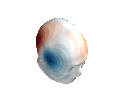
%% Compute potential

U_sph = potential( p, alpha, np.zeros(alpha.shape), lmax=lmax, normalization=”energy”, R=R )

U_suh = c.U_coupling(p) @ s

# evoked1 = evoked.copy()
# evoked1.data[:, :] = np.tile(U_sph.T, (evoked.times.shape[0], 1)).T
# evoked1.plot_topomap(times=0.080, ch_type="mag")

# evoked1 = evoked.copy()
# evoked1.data[:, :] = np.tile(U_suh.T, (evoked.times.shape[0], 1)).T
# evoked1.plot_topomap(times=0.080, ch_type="mag")

from bfieldtools.utils import load_example_mesh
from bfieldtools.mesh_calculus import gradient

plane = load_example_mesh("10x10_plane_hires")
scaling_factor = 0.03
plane.apply_scale(scaling_factor)
# Rotate to x-plane
t = np.eye(4)
theta = np.pi / 2 * 1.2
t[1:3, 1:3] = np.array(
    [[np.cos(theta), np.sin(theta)], [-np.sin(theta), np.cos(theta)]]
)
plane.apply_transform(t)

c.U_coupling.reset()
U_suh = c.U_coupling(plane.vertices) @ a
# Adapt mesh to the function and calculate new points
for i in range(2):
    g = np.linalg.norm(gradient(U_suh, plane), axis=0)
    face_ind = np.flatnonzero(g > g.max() * 0.05)
    plane = plane.subdivide(face_ind)
    U_suh = c.U_coupling(plane.vertices) @ a

U_sph = potential(
    plane.vertices, alpha, np.zeros(alpha.shape), lmax=lmax, normalization="energy", R=R
)

Out:

Computing scalar potential coupling matrix, 2562 vertices by 1592 target points... took 4.62 seconds.
Computing scalar potential coupling matrix, 2562 vertices by 819 target points... took 2.52 seconds.
Computing scalar potential coupling matrix, 2562 vertices by 867 target points... took 2.67 seconds.

# Mask inside/outside using solid angle
mask = abs(c.U_coupling.matrix.sum(axis=1)) < 1e-6
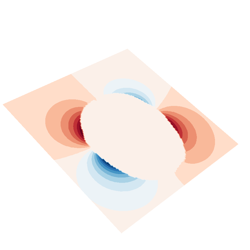
f = plot_data_on_vertices(plane, U_suh * mask, ncolors=15)
# plot_mesh(mesh, figure=f)
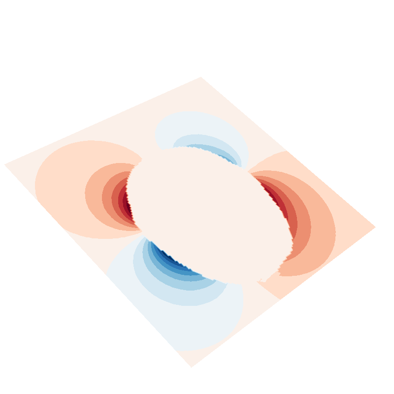
f = plot_data_on_vertices(plane, U_sph * mask, ncolors=15)
# plot_mesh(mesh, figure=f)
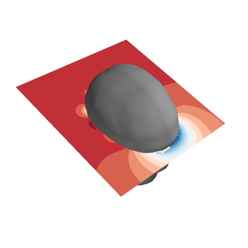
f = plot_data_on_vertices(plane, (U_suh - U_sph) * mask, ncolors=15)
plot_mesh(mesh, figure=f)

• 
• 
• 

Out:

<mayavi.modules.surface.Surface object at 0x7f94d8c1ad70>

Estimated memory usage: 1298 MB