Field interpolation example using equivalent surface currents

import numpy as np
from bfieldtools.mesh_conductor import MeshConductor, StreamFunction
from mayavi import mlab
import trimesh

import mne

PLOT = True
SAVE_FIGURES = True
IMPORT_MNE_DATA = True

SAVE_MNE_DATA = True
SAVE_DIR = "./MNE interpolation/"


from pyface.api import GUI

_gui = GUI()

First, let’s import the MEG data

if IMPORT_MNE_DATA:

    from mne.datasets import sample

    data_path = sample.data_path()
    fname = data_path + "/MEG/sample/sample_audvis-ave.fif"
    # Reading
    condition = "Left Auditory"
    evoked = mne.read_evokeds(fname, condition=condition, baseline=(None, 0), proj=True)
    evoked.pick_types(meg="mag")
    # evoked.plot(exclude=[], time_unit="s")

    i0, i1 = evoked.time_as_index(0.08)[0], evoked.time_as_index(0.09)[0]
    field = evoked.data[:, i0:i1].mean(axis=1)

    # Read BEM for surface geometry and transform to correct coordinate system
    import os.path as op

    subject = "sample"
    subjects_dir = op.join(data_path, "subjects")
    bem_fname = op.join(
        subjects_dir, subject, "bem", subject + "-5120-5120-5120-bem-sol.fif"
    )
    bem = mne.read_bem_solution(bem_fname)

    # Head mesh 0
    # Innerskull mesh 2
    surf_index = 2

    trans_fname = op.join(data_path, "MEG", "sample", "sample_audvis_raw-trans.fif")
    trans0 = mne.read_trans(trans_fname)
    R = trans0["trans"][:3, :3]
    t = trans0["trans"][:3, 3]
    # Surface from MRI to HEAD
    rr = (bem["surfs"][surf_index]["rr"] - t) @ R
    # Surface from HEAD to DEVICE
    trans1 = evoked.info["dev_head_t"]
    R = trans1["trans"][:3, :3]
    t = trans1["trans"][:3, 3]
    rr = (rr - t) @ R

    innerskull = trimesh.Trimesh(rr, bem["surfs"][surf_index]["tris"])

    surf_index = 0

    R = trans0["trans"][:3, :3]
    t = trans0["trans"][:3, 3]
    # Surface from MRI to HEAD
    rr = (bem["surfs"][surf_index]["rr"] - t) @ R
    # Surface from HEAD to DEVICE
    R = trans1["trans"][:3, :3]
    t = trans1["trans"][:3, 3]
    rr = (rr - t) @ R
    head = trimesh.Trimesh(rr, bem["surfs"][surf_index]["tris"])

    mesh = head

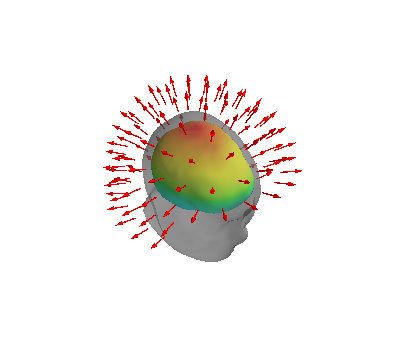
    # Sensor locations and directions in DEVICE coordinate system
    p = np.array(
        [
            ch["loc"][:3]
            for ch in evoked.info["chs"]
            if ch["ch_name"][-1] == "1" and ch["ch_name"][:3] == "MEG"
        ]
    )
    n = np.array(
        [
            ch["loc"][-3:]
            for ch in evoked.info["chs"]
            if ch["ch_name"][-1] == "1" and ch["ch_name"][:3] == "MEG"
        ]
    )

    if PLOT:
        # Plot sensor locations and directions
        fig = mlab.figure(bgcolor=(1, 1, 1))
        mlab.triangular_mesh(*innerskull.vertices.T, innerskull.faces)
        mlab.triangular_mesh(
            *head.vertices.T, head.faces, color=(0.5, 0.5, 0.5), opacity=0.5
        )
        mlab.quiver3d(*p.T, *n.T, mode="arrow")

        fig.scene.isometric_view()

        if SAVE_FIGURES:
            mlab.savefig(SAVE_DIR + "MEG_geometry.png", magnification=4, figure=fig)

    if SAVE_MNE_DATA:
        np.savez(
            SAVE_DIR + "mne_data.npz",
            mesh=head,
            p=p,
            n=n,
            vertices=head.vertices,
            faces=head.faces,
        )
        evoked.save(SAVE_DIR + "left_auditory-ave.fif")


else:

    with np.load(SAVE_DIR + "mne_data.npz", allow_pickle=True) as data:
        mesh = data["mesh"]
        p = data["p"]
        n = data["n"]
        mesh = trimesh.Trimesh(vertices=data["vertices"], faces=data["faces"])

    evoked = mne.Evoked(SAVE_DIR + "left_auditory-ave.fif")

Out:

Reading /home/rzetter/mne_data/MNE-sample-data/MEG/sample/sample_audvis-ave.fif ...
    Read a total of 4 projection items:
        PCA-v1 (1 x 102) active
        PCA-v2 (1 x 102) active
        PCA-v3 (1 x 102) active
        Average EEG reference (1 x 60) active
    Found the data of interest:
        t =    -199.80 ...     499.49 ms (Left Auditory)
        0 CTF compensation matrices available
        nave = 55 - aspect type = 100
Projections have already been applied. Setting proj attribute to True.
Applying baseline correction (mode: mean)
Loading surfaces...
Three-layer model surfaces loaded.

Loading the solution matrix...

Loaded linear_collocation BEM solution from /home/rzetter/mne_data/MNE-sample-data/subjects/sample/bem/sample-5120-5120-5120-bem-sol.fif

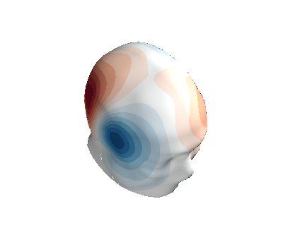
Fit the surface current for the auditory evoked response

c = MeshConductor(mesh_obj=mesh, basis_name="suh", N_suh=150)
M = c.mass

sensor_coupling = np.einsum("ijk,ij->ik", c.B_coupling(p), n)
# a = np.linalg.pinv(sensor_coupling, rcond=1e-15) @ field
ss = np.linalg.svd(sensor_coupling @ sensor_coupling.T, False, False)

# reg_exps = [0.5, 1, 2, 3, 4, 5, 6, 7, 8]
reg_exps = [1]
rel_errors = []

for reg_exp in reg_exps:
    _lambda = np.max(ss) * (10 ** (-reg_exp))
    # Laplacian in the suh basis is diagonal
    BB = sensor_coupling.T @ sensor_coupling + _lambda * (-c.laplacian) / np.max(
        abs(c.laplacian)
    )
    a = np.linalg.solve(BB, sensor_coupling.T @ field)
    s = StreamFunction(a, c)
    b_filt = sensor_coupling @ s

    rel_error = np.linalg.norm(b_filt - field) / np.linalg.norm(field)
    print("Relative error:", rel_error * 100, "%")
    rel_errors.append(rel_error)

    if PLOT:
        fig = mlab.figure(bgcolor=(1, 1, 1))
        surf = s.plot(False, figure=fig)
        surf.actor.mapper.interpolate_scalars_before_mapping = True
        surf.module_manager.scalar_lut_manager.number_of_colors = 16

        if SAVE_FIGURES:
            mlab.savefig(
                SAVE_DIR + "SUH_scalp_streamfunction.png", magnification=4, figure=fig
            )

Out:

Calculating surface harmonics expansion...
Computing the laplacian matrix...
Computing the mass matrix...
Closed mesh or Neumann BC, leaving out the constant component
Computing the mass matrix...
Computing magnetic field coupling matrix, 2562 vertices by 102 target points... took 0.23 seconds.
Computing the laplacian matrix...
Relative error: 2.0549237013162216 %

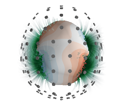
Interpolate MEG data to the sensor surface

from bfieldtools.utils import load_example_mesh

helmet = load_example_mesh("meg_helmet", process=False)
# Bring the surface roughly to the correct place
helmet.vertices[:, 2] -= 0.05

# Reset coupling by hand
c.B_coupling.reset()
mlab.figure(bgcolor=(1, 1, 1))
B_surf = np.sum(
    c.B_coupling(helmet.vertices) * helmet.vertex_normals[:, :, None], axis=1
)

if PLOT:
    fig = mlab.quiver3d(*p.T, *n.T, mode="arrow")
    scalars = B_surf @ s
    surf = mlab.triangular_mesh(
        *helmet.vertices.T, helmet.faces, scalars=scalars, colormap="seismic"
    )
    surf.actor.mapper.interpolate_scalars_before_mapping = True
    surf.module_manager.scalar_lut_manager.number_of_colors = 15

    if SAVE_FIGURES:
        mlab.savefig(
            SAVE_DIR + "SUH_sensors_streamfunction.png", magnification=4, figure=fig
        )

Out:

Computing magnetic field coupling matrix, 2562 vertices by 2044 target points... took 1.36 seconds.

Calculate magnetic field in volumetric grid

Nvol = 30
x = np.linspace(-0.125, 0.125, Nvol)
vol_points = np.array(np.meshgrid(x, x, x, indexing="ij")).reshape(3, -1).T
# mlab.points3d(*vol_points.T)

c.B_coupling.reset()
Bvol_coupling = c.B_coupling(vol_points, Nchunks=100, analytic=True)
s = StreamFunction(a, c)
# s = StreamFunction(a, c)
Bvol = Bvol_coupling @ s

Out:

Computing magnetic field coupling matrix analytically, 2562 vertices by 27000 target points... took 82.12 seconds.

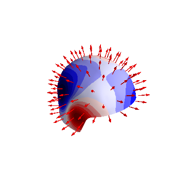
Now, plot the computed magnetic field using streamlines

if PLOT:
    from bfieldtools.mesh_calculus import gradient

    fig = mlab.figure(bgcolor=(1, 1, 1))

    surf = s.plot(False, figure=fig)
    surf.actor.mapper.interpolate_scalars_before_mapping = True
    surf.module_manager.scalar_lut_manager.number_of_colors = 16

    vecs = mlab.pipeline.vector_field(
        *vol_points.T.reshape(3, Nvol, Nvol, Nvol), *Bvol.T.reshape(3, Nvol, Nvol, Nvol)
    )
    vecnorm = mlab.pipeline.extract_vector_norm(vecs)

    seed_points = mesh.vertices[mesh.faces].mean(axis=1) - 0.01 * mesh.face_normals

    seed_vals = c.basis @ c.inductance @ s
    seed_vals_grad = np.linalg.norm(gradient(seed_vals, c.mesh), axis=0)

    seed_vals = abs(seed_vals[mesh.faces].mean(axis=1)) ** 2
    seed_vals[seed_vals_grad > seed_vals_grad.max() / 1.8] = 0

    Npoints = 500
    seed_inds = np.random.choice(
        np.arange(len(seed_vals)), Npoints, False, seed_vals / seed_vals.sum()
    )

    seed_points = seed_points[seed_inds]

    streams = []

    for pi in seed_points:
        streamline = mlab.pipeline.streamline(
            vecnorm,
            integration_direction="both",
            colormap="BuGn",
            seed_visible=False,
            seedtype="point",
        )
        streamline.seed.widget.position = pi
        streamline.stream_tracer.terminal_speed = 3e-13
        streamline.stream_tracer.maximum_propagation = 0.1
        streamline.actor.property.render_lines_as_tubes = True
        streamline.actor.property.line_width = 4.0
        streams.append(streamline)

    # Custom colormap with alpha channel
    streamine = streams[0]
    lut = streamline.module_manager.scalar_lut_manager.lut.table.to_array()
    lut[:, -1] = np.linspace(0, 255, 256)
    streamline.module_manager.scalar_lut_manager.lut.table = lut
    streamline.module_manager.scalar_lut_manager.data_range = np.array(
        [1.0e-13, 1.0e-12]
    )

    for streamline in streams:
        streamline.stream_tracer.terminal_speed = 1e-13
        streamline.seed.widget.hot_spot_size = 0.1
        streamline.stream_tracer.initial_integration_step = 0.01
        streamline.stream_tracer.minimum_integration_step = 0.1

    sensors = mlab.quiver3d(*p.T, *n.T, mode="cylinder")
    sensors.glyph.glyph_source.glyph_source.height = 0.1
    sensors.actor.property.color = (0.5, 0.5, 0.5)
    sensors.actor.mapper.scalar_visibility = False
    sensors.glyph.glyph_source.glyph_source.resolution = 32
    sensors.glyph.glyph.scale_factor = 0.03
    # sensors.glyph.glyph_source.glyph_source.shaft_radius = 0.05

    fig.scene.camera.position = [
        0.637392177469018,
        0.07644693029292644,
        -0.07183513804689762,
    ]
    fig.scene.camera.focal_point = [
        -6.413459777832031e-05,
        0.01716560870409012,
        -0.0229007127850005,
    ]
    fig.scene.camera.view_angle = 30.0
    fig.scene.camera.view_up = [
        0.04390624852005244,
        0.3114421192517664,
        0.9492502555685007,
    ]
    fig.scene.camera.clipping_range = [0.3366362817578398, 1.0281065506557443]
    fig.scene.camera.compute_view_plane_normal()

    while fig.scene.light_manager is None:
        _gui.process_events()

    camera_light = fig.scene.light_manager.lights[0]
    camera_light.intensity = 0.7

    if SAVE_FIGURES:
        mlab.savefig(
            SAVE_DIR + "SUH_streamlines_lateral.png", figure=fig, magnification=4
        )

    fig.scene.camera.position = [
        -6.413459777832031e-05,
        0.01716560870409012,
        0.6191735842078244,
    ]
    fig.scene.camera.focal_point = [
        -6.413459777832031e-05,
        0.01716560870409012,
        -0.0229007127850005,
    ]
    fig.scene.camera.view_angle = 30.0
    fig.scene.camera.view_up = [0.0, 1.0, 0.0]
    fig.scene.camera.clipping_range = [0.3381552363433513, 1.0261944997830243]
    fig.scene.camera.compute_view_plane_normal()

    if SAVE_FIGURES:
        mlab.savefig(
            SAVE_DIR + "SUH_streamlines_coronal.png", figure=fig, magnification=4
        )

Out:

Computing the inductance matrix...
Computing self-inductance matrix using rough quadrature (degree=2).              For higher accuracy, set quad_degree to 4 or more.
Estimating 24058 MiB required for 2562 by 2562 vertices...
Computing inductance matrix in 80 chunks (7035 MiB memory free),              when approx_far=True using more chunks is faster...
Computing triangle-coupling matrix
Inductance matrix computation took 10.99 seconds.

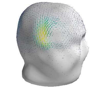
Finally, plot the surface current density itself

fig = mlab.figure(bgcolor=(1, 1, 1))
grad_s = gradient(c.basis @ s, mesh, rotated=True)
q = mlab.quiver3d(
    *(mesh.vertices[mesh.faces].mean(axis=1).T),
    *grad_s,
    colormap="viridis",
    mode="arrow"
)

mlab.triangular_mesh(*head.vertices.T, head.faces, color=(0.8, 0.8, 0.8), opacity=1.0)

fig.scene.camera.position = [
    0.4987072212753703,
    0.06469079487766746,
    -0.0014732384935239248,
]
fig.scene.camera.focal_point = [
    0.0018187984824180603,
    0.012344694641686624,
    -0.04367139294433087,
]
fig.scene.camera.view_angle = 30.0
fig.scene.camera.view_up = [
    -0.10720122151366927,
    0.23975383168819672,
    0.9648968848000314,
]
fig.scene.camera.clipping_range = [0.28329092545021717, 0.7772019991936254]
fig.scene.camera.compute_view_plane_normal()

if SAVE_FIGURES:
    mlab.savefig(
        SAVE_DIR + "SUH_surface_currents_lateral.png", figure=fig, magnification=4
    )

Estimated memory usage: 8527 MB