Note
Click here to download the full example code
Coil with minimal eddy currents
Compact example of design of a cylindrical coil surrounded by a RF shield, i.e. a conductive surface. The effects of eddy currents due to inductive interaction with the shield is minimized
PLOT = True
SAVE_FIGURES = False
SAVE_PATH = "./Minimal eddy current coil/"


import numpy as np
from mayavi import mlab
import trimesh


from bfieldtools.mesh_conductor import MeshConductor

from bfieldtools.coil_optimize import optimize_streamfunctions
from bfieldtools.contour import scalar_contour
from bfieldtools.viz import plot_3d_current_loops, plot_data_on_vertices

import pkg_resources

from pyface.api import GUI

_gui = GUI()


# Set unit, e.g. meter or millimeter.
# This doesn't matter, the problem is scale-invariant
scaling_factor = 1


# Load example coil mesh that is centered on the origin
coilmesh = trimesh.load(
    file_obj=pkg_resources.resource_filename(
        "bfieldtools", "example_meshes/open_cylinder.stl"
    ),
    process=True,
)

angle = np.pi / 2
rotation_matrix = np.array(
    [
        [np.cos(angle), 0, np.sin(angle), 0],
        [0, 1, 0, 0],
        [-np.sin(angle), 0, np.cos(angle), 0],
        [0, 0, 0, 1],
    ]
)

coilmesh.apply_transform(rotation_matrix)

coilmesh1 = coilmesh.copy()
# coilmesh1.apply_scale(1.3)

coilmesh2 = coilmesh.copy()

# coilmesh1 = coilmesh.union(coilmesh1)
# coilmesh1 = coilmesh1.subdivide().subdivide()
# coilmesh2 = coilmesh.subdivide()


# Create mesh class object
coil = MeshConductor(
    verts=coilmesh1.vertices * 0.75,
    tris=coilmesh1.faces,
    fix_normals=True,
    basis_name="suh",
    N_suh=400,
)


def alu_sigma(T):
    ref_T = 293  # K
    ref_rho = 2.82e-8  # ohm*meter
    alpha = 0.0039  # 1/K

    rho = alpha * (T - ref_T) * ref_rho + ref_rho

    return 1 / rho


resistivity = 1 / alu_sigma(T=293)  # room-temp Aluminium
thickness = 0.5e-3  # 0.5 mm thick


# Separate object for shield geometry
shield = MeshConductor(
    verts=coilmesh2.vertices.copy() * 1.1,
    tris=coilmesh2.faces.copy(),
    fix_normals=True,
    basis_name="inner",
    resistivity=resistivity,
    thickness=thickness,
)
# shield.mesh.vertices[:,2] -= 3
# shield.mesh.vertices *= np.array([1.2, 1.2, 1.2])
#
# angle = np.pi/2
# rotation_matrix = np.array([[np.cos(angle), 0, np.sin(angle), 0],
#                              [0, 1, 0, 0],
#                              [-np.sin(angle), 0, np.cos(angle), 0],
#                              [0, 0, 0, 1]
#                              ])
#
# shield.mesh.apply_transform(rotation_matrix)
#
# shield.mesh = shield.mesh.subdivide()
Out:
Calculating surface harmonics expansion...
Computing the laplacian matrix...
Computing the mass matrix...
Set up target points and plot geometry
# Here, the target points are on a volumetric grid within a sphere

center = np.array([0, 0, 0])

sidelength = 0.25 * scaling_factor
n = 12
xx = np.linspace(-sidelength / 2, sidelength / 2, n)
yy = np.linspace(-sidelength / 2, sidelength / 2, n)
zz = np.linspace(-sidelength / 2, sidelength / 2, n)
X, Y, Z = np.meshgrid(xx, yy, zz, indexing="ij")

x = X.ravel()
y = Y.ravel()
z = Z.ravel()

target_points = np.array([x, y, z]).T

# Turn cube into sphere by rejecting points "in the corners"
target_points = (
    target_points[np.linalg.norm(target_points, axis=1) < sidelength / 2] + center
)


# Plot coil, shield and target points
if PLOT:
    f = mlab.figure(None, bgcolor=(1, 1, 1), fgcolor=(0.5, 0.5, 0.5), size=(800, 800))
    coil.plot_mesh(figure=f, opacity=0.2)
    shield.plot_mesh(figure=f, opacity=0.2)
    mlab.points3d(*target_points.T)
Compute C matrices that are used to compute the generated magnetic field
mutual_inductance = coil.mutual_inductance(shield)

# Take into account the field produced by currents induced into the shield
# NB! This expression is for instantaneous step-function switching of coil current, see Eq. 18 in G.N. Peeren, 2003.

shield.M_coupling = np.linalg.solve(-shield.inductance, mutual_inductance.T)
secondary_C = shield.B_coupling(target_points) @ -shield.M_coupling
Out:
Estimating 69923 MiB required for 4764 by 4764 vertices...
Computing inductance matrix in 160 chunks (9444 MiB memory free),              when approx_far=True using more chunks is faster...
Computing triangle-coupling matrix
Computing the inductance matrix...
Computing self-inductance matrix using rough quadrature (degree=2).              For higher accuracy, set quad_degree to 4 or more.
Estimating 69923 MiB required for 4764 by 4764 vertices...
Computing inductance matrix in 160 chunks (8915 MiB memory free),              when approx_far=True using more chunks is faster...
Computing triangle-coupling matrix
Inductance matrix computation took 31.49 seconds.
Computing magnetic field coupling matrix, 4764 vertices by 672 target points... took 0.99 seconds.
Create bfield specifications used when optimizing the coil geometry
# The absolute target field amplitude is not of importance,
# and it is scaled to match the C matrix in the optimization function

target_field = np.zeros(target_points.shape)
target_field[:, 1] = target_field[:, 1] + 1


target_spec = {
    "coupling": coil.B_coupling(target_points),
    "abs_error": 0.01,
    "target": target_field,
}


from scipy.linalg import eigh

l, U = eigh(shield.resistance, shield.inductance, eigvals=(0, 500))
#
# U = np.zeros((shield.inductance.shape[0], len(li)))
# U[shield.inner_verts, :] = Ui


#
# plt.figure()
# plt.plot(1/li)


# shield.M_coupling = np.linalg.solve(-shield.inductance, mutual_inductance.T)
# secondary_C = shield.B_coupling(target_points) @ -shield.M_coupling


#
# tmin, tmax = 0.001, 0.001
# Fs=10000

time = [0.001, 0.003, 0.005]
eddy_error = [0.05, 0.01, 0.0025]
# time_decay = U @ np.exp(-l[None, :]*time[:, None]) @ np.pinv(U)

time_decay = np.zeros(
    (len(time), shield.inductance.shape[0], shield.inductance.shape[1])
)

induction_spec = []


Uinv = np.linalg.pinv(U)
for idx, t in enumerate(time):
    time_decay = U @ np.diag(np.exp(-l * t)) @ Uinv
    eddy_coupling = shield.B_coupling(target_points) @ time_decay @ shield.M_coupling
    induction_spec.append(
        {
            "coupling": eddy_coupling,
            "abs_error": eddy_error[idx],
            "rel_error": 0,
            "target": np.zeros_like(target_field),
        }
    )
Out:
Computing magnetic field coupling matrix, 4764 vertices by 672 target points... took 1.03 seconds.
Computing the resistance matrix...
Run QP solver
import mosek

coil.s, prob = optimize_streamfunctions(
    coil,
    [target_spec] + induction_spec,
    objective="minimum_inductive_energy",
    solver="MOSEK",
    solver_opts={"mosek_params": {mosek.iparam.num_threads: 8}},
)

from bfieldtools.mesh_conductor import StreamFunction

shield.induced_s = StreamFunction(shield.M_coupling @ coil.s, shield)
Out:
Computing the inductance matrix...
Computing self-inductance matrix using rough quadrature (degree=2).              For higher accuracy, set quad_degree to 4 or more.
Estimating 69923 MiB required for 4764 by 4764 vertices...
Computing inductance matrix in 180 chunks (8207 MiB memory free),              when approx_far=True using more chunks is faster...
Computing triangle-coupling matrix
Inductance matrix computation took 30.40 seconds.
Passing problem to solver...


Problem
  Name                   :
  Objective sense        : min
  Type                   : CONIC (conic optimization problem)
  Constraints            : 16530
  Cones                  : 1
  Scalar variables       : 803
  Matrix variables       : 0
  Integer variables      : 0

Optimizer started.
Problem
  Name                   :
  Objective sense        : min
  Type                   : CONIC (conic optimization problem)
  Constraints            : 16530
  Cones                  : 1
  Scalar variables       : 803
  Matrix variables       : 0
  Integer variables      : 0

Optimizer  - threads                : 8
Optimizer  - solved problem         : the dual
Optimizer  - Constraints            : 401
Optimizer  - Cones                  : 1
Optimizer  - Scalar variables       : 16530             conic                  : 402
Optimizer  - Semi-definite variables: 0                 scalarized             : 0
Factor     - setup time             : 0.28              dense det. time        : 0.00
Factor     - ML order time          : 0.00              GP order time          : 0.00
Factor     - nonzeros before factor : 8.06e+04          after factor           : 8.06e+04
Factor     - dense dim.             : 0                 flops                  : 1.34e+09
ITE PFEAS    DFEAS    GFEAS    PRSTATUS   POBJ              DOBJ              MU       TIME
0   3.2e+01  1.0e+00  2.0e+00  0.00e+00   0.000000000e+00   -1.000000000e+00  1.0e+00  1.56
1   1.7e+01  5.2e-01  1.2e+00  -6.51e-01  8.755235291e+01   8.717745151e+01   5.2e-01  1.64
2   1.0e+01  3.2e-01  7.5e-01  -3.65e-01  3.120153253e+02   3.119964808e+02   3.2e-01  1.71
3   7.2e+00  2.2e-01  5.4e-01  -9.84e-02  6.857677666e+02   6.859575059e+02   2.2e-01  1.79
4   5.5e+00  1.7e-01  4.3e-01  -2.59e-01  1.163962871e+03   1.164387060e+03   1.7e-01  1.86
5   1.9e+00  5.8e-02  1.5e-01  -2.36e-01  7.480098289e+03   7.481027404e+03   5.8e-02  1.94
6   6.8e-01  2.1e-02  4.7e-02  1.04e-01   1.627369627e+04   1.627454019e+04   2.1e-02  2.02
7   3.5e-01  1.1e-02  1.9e-02  7.70e-01   2.132852436e+04   2.132909581e+04   1.1e-02  2.12
8   3.2e-01  9.8e-03  1.7e-02  5.09e-01   2.209800849e+04   2.209853836e+04   9.8e-03  2.20
9   1.5e-01  4.5e-03  5.9e-03  6.46e-01   2.619385305e+04   2.619417789e+04   4.5e-03  2.27
10  4.2e-02  1.3e-03  1.1e-03  7.82e-01   2.972842030e+04   2.972856480e+04   1.3e-03  2.39
11  2.2e-02  6.8e-04  4.5e-04  8.03e-01   3.075144691e+04   3.075153484e+04   6.8e-04  2.45
12  8.2e-04  2.5e-05  3.8e-06  8.85e-01   3.207619890e+04   3.207620363e+04   2.5e-05  2.55
13  1.4e-04  4.2e-06  2.6e-07  9.95e-01   3.213108587e+04   3.213108671e+04   4.2e-06  2.62
14  7.1e-06  6.1e-08  1.9e-09  9.99e-01   3.214223523e+04   3.214223526e+04   6.2e-09  2.70
15  7.1e-06  6.1e-08  1.9e-09  1.00e+00   3.214223523e+04   3.214223526e+04   6.2e-09  2.94
16  6.7e-06  4.6e-08  1.1e-09  1.00e+00   3.214223932e+04   3.214223934e+04   4.6e-09  3.10
17  1.3e-05  3.4e-08  6.2e-10  1.00e+00   3.214224239e+04   3.214224238e+04   3.5e-09  3.27
18  5.7e-06  3.2e-08  4.7e-10  1.00e+00   3.214224297e+04   3.214224298e+04   3.3e-09  3.44
19  5.7e-06  3.2e-08  4.7e-10  1.00e+00   3.214224297e+04   3.214224298e+04   3.3e-09  3.68
20  5.7e-06  3.2e-08  4.7e-10  1.00e+00   3.214224297e+04   3.214224298e+04   3.3e-09  3.91
Optimizer terminated. Time: 4.24


Interior-point solution summary
  Problem status  : PRIMAL_AND_DUAL_FEASIBLE
  Solution status : OPTIMAL
  Primal.  obj: 3.2142242969e+04    nrm: 6e+04    Viol.  con: 5e-08    var: 0e+00    cones: 0e+00
  Dual.    obj: 3.2142242978e+04    nrm: 4e+05    Viol.  con: 0e+00    var: 5e-07    cones: 0e+00
Plot coil windings and target points
loops = scalar_contour(coil.mesh, coil.s.vert, N_contours=6)

# loops = [simplify_contour(loop, min_edge=1e-2, angle_threshold=2e-2, smooth=True) for loop in loops]

# loops = [loop for loop in loops if loop is not None]
if PLOT:
    f = mlab.figure(None, bgcolor=(1, 1, 1), fgcolor=(0.5, 0.5, 0.5), size=(600, 500))
    mlab.clf()

    plot_3d_current_loops(loops, colors="auto", figure=f, tube_radius=0.005)

    B_target = coil.B_coupling(target_points) @ coil.s

    mlab.quiver3d(*target_points.T, *B_target.T)

    #    plot_data_on_vertices(shield.mesh, shield.induced_s.vert, ncolors=256, figure=f, opacity=0.5, cull_back=True)
    #    plot_data_on_vertices(shield.mesh, shield.induced_s.vert, ncolors=256, figure=f, opacity=1, cull_front=True)

    shield.plot_mesh(
        representation="surface",
        opacity=0.5,
        cull_back=True,
        color=(0.8, 0.8, 0.8),
        figure=f,
    )
    shield.plot_mesh(
        representation="surface",
        opacity=1,
        cull_front=True,
        color=(0.8, 0.8, 0.8),
        figure=f,
    )

    f.scene.camera.parallel_projection = 1

    f.scene.camera.zoom(1.4)

    while f.scene.light_manager is None:
        _gui.process_events()

    if SAVE_FIGURES:
        mlab.savefig(SAVE_PATH + "eddy_yes.png", figure=f, magnification=4)
        mlab.close()
# mlab.triangular_mesh(*shield.mesh.vertices.T, shield.mesh.faces, scalars=shield.induced_I)

# mlab.title('Coils which minimize the transient effects of conductive shield')
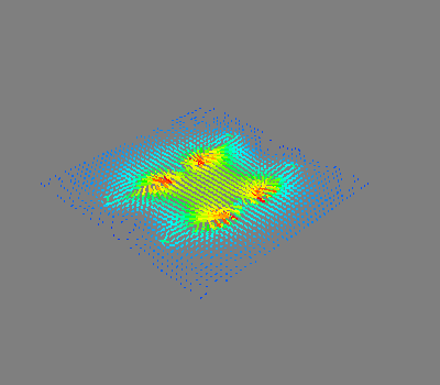
Plot cross-section of magnetic field and magnetic potential of the discretized loops
import matplotlib.pyplot as plt

x = y = np.linspace(-1, 1, 40)
X, Y = np.meshgrid(x, y, indexing="ij")


points = np.zeros((X.flatten().shape[0], 3))
points[:, 0] = X.flatten()
points[:, 1] = Y.flatten()

B = coil.B_coupling(points) @ coil.s


mlab.quiver3d(*points.T, *B.T)

# U = U.reshape(x.shape[0], y.shape[0])
# B = B.T[:2].reshape(2, x.shape[0], y.shape[0])

# from bfieldtools.viz import plot_cross_section

# lw = np.sqrt(B[0] ** 2 + B[1] ** 2)

# lw = 2 * lw / np.max(lw)

# plot_cross_section(X, Y, U, log=False, contours=False)

# seed_points = points[:, :2] * 0.3

# plt.streamplot(
#     x,
#     y,
#     B[0],
#     B[1],
#     density=2,
#     linewidth=lw,
#     color="k",
#     integration_direction="both",
#     start_points=seed_points,
# )


# plt.tight_layout()
Out:
Computing magnetic field coupling matrix, 4764 vertices by 1600 target points... took 1.87 seconds.

<mayavi.modules.vectors.Vectors object at 0x7f94c70b8230>
For comparison, let’s see how the coils look when we ignore the conducting shield
coil.unshielded_s, coil.unshielded_prob = optimize_streamfunctions(
    coil,
    [target_spec],
    objective="minimum_inductive_energy",
    solver="MOSEK",
    solver_opts={"mosek_params": {mosek.iparam.num_threads: 8}},
)

shield.unshielded_induced_s = StreamFunction(
    shield.M_coupling @ coil.unshielded_s, shield
)

loops = scalar_contour(coil.mesh, coil.unshielded_s.vert, N_contours=6)
if PLOT:
    f = mlab.figure(None, bgcolor=(1, 1, 1), fgcolor=(0.5, 0.5, 0.5), size=(600, 500))
    mlab.clf()

    plot_3d_current_loops(loops, colors="auto", figure=f, tube_radius=0.005)

    B_target_unshielded = coil.B_coupling(target_points) @ coil.unshielded_s

    mlab.quiver3d(*target_points.T, *B_target_unshielded.T)
    #
    #    plot_data_on_vertices(shield.mesh, shield.unshielded_induced_s.vert,  ncolors=256, figure=f, opacity=0.5, cull_back=True)
    #    plot_data_on_vertices(shield.mesh, shield.unshielded_induced_s.vert, ncolors=256, figure=f, opacity=1, cull_front=True)

    shield.plot_mesh(
        representation="surface",
        opacity=0.5,
        cull_back=True,
        color=(0.8, 0.8, 0.8),
        figure=f,
    )
    shield.plot_mesh(
        representation="surface",
        opacity=1,
        cull_front=True,
        color=(0.8, 0.8, 0.8),
        figure=f,
    )

    f.scene.camera.parallel_projection = 1

    f.scene.camera.zoom(1.4)

    while f.scene.light_manager is None:
        _gui.process_events()

    if SAVE_FIGURES:
        mlab.savefig(SAVE_PATH + "eddy_no.png", figure=f, magnification=4)
        mlab.close()
Out:
Passing problem to solver...


Problem
  Name                   :
  Objective sense        : min
  Type                   : CONIC (conic optimization problem)
  Constraints            : 4434
  Cones                  : 1
  Scalar variables       : 803
  Matrix variables       : 0
  Integer variables      : 0

Optimizer started.
Problem
  Name                   :
  Objective sense        : min
  Type                   : CONIC (conic optimization problem)
  Constraints            : 4434
  Cones                  : 1
  Scalar variables       : 803
  Matrix variables       : 0
  Integer variables      : 0

Optimizer  - threads                : 8
Optimizer  - solved problem         : the dual
Optimizer  - Constraints            : 401
Optimizer  - Cones                  : 1
Optimizer  - Scalar variables       : 4434              conic                  : 402
Optimizer  - Semi-definite variables: 0                 scalarized             : 0
Factor     - setup time             : 0.06              dense det. time        : 0.00
Factor     - ML order time          : 0.00              GP order time          : 0.00
Factor     - nonzeros before factor : 8.06e+04          after factor           : 8.06e+04
Factor     - dense dim.             : 0                 flops                  : 3.67e+08
ITE PFEAS    DFEAS    GFEAS    PRSTATUS   POBJ              DOBJ              MU       TIME
0   3.2e+01  1.0e+00  2.0e+00  0.00e+00   0.000000000e+00   -1.000000000e+00  1.0e+00  0.38
1   2.5e+01  7.8e-01  2.4e-01  2.19e+00   3.606895285e+01   3.532195174e+01   7.8e-01  0.40
2   1.4e+00  4.2e-02  6.7e-03  1.32e+00   4.778977359e+01   4.776570562e+01   4.2e-02  0.43
3   9.6e-02  3.0e-03  8.7e-05  1.06e+00   4.681593779e+01   4.681405007e+01   3.0e-03  0.45
4   1.9e-02  5.8e-04  8.8e-06  1.00e+00   4.676836958e+01   4.676801715e+01   5.8e-04  0.47
5   1.7e-04  5.1e-06  8.1e-09  1.00e+00   4.677179327e+01   4.677179029e+01   5.1e-06  0.50
6   6.2e-06  1.9e-07  5.8e-11  1.00e+00   4.677191103e+01   4.677191092e+01   1.9e-07  0.53
7   3.1e-06  9.5e-08  2.2e-11  1.00e+00   4.677191365e+01   4.677191359e+01   9.5e-08  0.56
8   1.5e-06  4.8e-08  5.7e-12  1.00e+00   4.677191496e+01   4.677191494e+01   4.8e-08  0.60
9   7.7e-07  2.4e-08  2.0e-12  1.00e+00   4.677191562e+01   4.677191561e+01   2.4e-08  0.63
Optimizer terminated. Time: 0.65


Interior-point solution summary
  Problem status  : PRIMAL_AND_DUAL_FEASIBLE
  Solution status : OPTIMAL
  Primal.  obj: 4.6771915620e+01    nrm: 9e+01    Viol.  con: 8e-09    var: 0e+00    cones: 0e+00
  Dual.    obj: 4.6771915610e+01    nrm: 4e+01    Viol.  con: 1e-07    var: 2e-10    cones: 0e+00
Out:
<mayavi.modules.vectors.Vectors object at 0x7f94c70066b0>
Finally, let’s compare the time-courses
tmin, tmax = 0, 0.025
Fs = 2000

time = np.linspace(tmin, tmax, int(Fs * (tmax - tmin) + 1))

# time_decay = U @ np.exp(-l[None, :]*time[:, None]) @ np.pinv(U)

time_decay = np.zeros(
    (len(time), shield.inductance.shape[0], shield.inductance.shape[1])
)

Uinv = np.linalg.pinv(U)
for idx, t in enumerate(time):
    time_decay[idx] = U @ np.diag(np.exp(-l * t)) @ Uinv


B_t = shield.B_coupling(target_points) @ (time_decay @ shield.induced_s).T

unshieldedB_t = (
    shield.B_coupling(target_points) @ (time_decay @ shield.unshielded_induced_s).T
)

import matplotlib.pyplot as plt

if PLOT and SAVE_FIGURES:
    fig, ax = plt.subplots(1, 1, sharex=True, figsize=(8, 4))
    ax.plot(
        time * 1e3,
        np.mean(np.linalg.norm(B_t, axis=1), axis=0).T,
        "k-",
        label="Constrained",
        linewidth=1.5,
    )
    # ax[0].set_title('Eddy currents minimized')
    ax.set_ylabel("Transient field amplitude")
    ax.semilogy(
        time * 1e3,
        np.mean(np.linalg.norm(unshieldedB_t, axis=1), axis=0).T,
        "k--",
        label="Ignored",
        linewidth=1.5,
    )
    # ax[1].set_title('Eddy currents ignored')
    ax.set_xlabel("Time (ms)")
    # ax[1].set_ylabel('Transient field amplitude')

    ax.set_ylim(1e-4, 0.5)
    ax.set_xlim(0, 25)
    #
    #    ax.spines['top'].set_visible(False)
    #    ax.spines['right'].set_visible(False)

    plt.grid(which="both", axis="y", alpha=0.1)

    plt.legend()
    fig.tight_layout()

    ax.vlines([1, 5, 10, 20], 1e-4, 0.5, alpha=0.1, linewidth=3, color="r")

    plt.savefig(SAVE_PATH + "eddy_transient.pdf")


from bfieldtools.mesh_calculus import gradient

from mayavi.api import Engine

engine = Engine()
engine.start()


if PLOT and SAVE_FIGURES:

    for plot_time_idx in [2, 10, 20, 40]:
        # EDDY CURRENTS MINIMIZED
        f = mlab.figure(
            None, bgcolor=(1, 1, 1), fgcolor=(0.5, 0.5, 0.5), size=(600, 500)
        )

        mlab.test_points3d()
        mlab.clf()

        shield.plot_mesh(
            representation="surface", color=(0.8, 0.8, 0.8), opacity=1, figure=f
        )

        s = np.zeros((shield.mesh.vertices.shape[0],))
        s[shield.inner_vertices] = time_decay[plot_time_idx] @ shield.induced_s

        #        mlab.quiver3d(*shield.mesh.triangles_center.T, *gradient(s, shield.mesh, rotated=True), colormap='viridis')

        plot_data_on_vertices(
            shield.mesh,
            s,
            ncolors=256,
            figure=f,
            opacity=1,
            cull_back=False,
            colormap="RdBu",
        )

        surface1 = engine.scenes[0].children[1].children[0].children[0].children[0]
        surface1.enable_contours = True
        surface1.contour.number_of_contours = 20
        surface1.actor.property.line_width = 10.0

        f.scene.camera.parallel_projection = 1
        f.scene.isometric_view()

        #        mlab.view(90,0)
        #        mlab.roll(180)
        f.scene.camera.zoom(1.4)

        while f.scene.light_manager is None:
            _gui.process_events()

        f.scene.light_manager.light_mode = "raymond"

        mlab.savefig(
            SAVE_PATH + "shield_eddy_yes_time_%.3f.png" % time[plot_time_idx],
            figure=f,
            magnification=2,
        )
        mlab.close()

    for plot_time_idx in [2, 10, 20, 40]:
        # EDDY CURRENTS IGNORED
        f = mlab.figure(
            None, bgcolor=(1, 1, 1), fgcolor=(0.5, 0.5, 0.5), size=(600, 500)
        )

        shield.plot_mesh(
            representation="surface", color=(0.8, 0.8, 0.8), opacity=1, figure=f
        )

        s_u = np.zeros((shield.mesh.vertices.shape[0],))
        s_u[shield.inner_vertices] = (
            time_decay[plot_time_idx] @ shield.unshielded_induced_s
        )

        #        mlab.quiver3d(*shield.mesh.triangles_center.T, *gradient(s_u, shield.mesh, rotated=True), colormap='viridis')

        plot_data_on_vertices(
            shield.mesh,
            s_u,
            ncolors=256,
            figure=f,
            opacity=1,
            cull_back=False,
            colormap="RdBu",
        )

        surface1 = engine.scenes[0].children[1].children[0].children[0].children[0]
        surface1.enable_contours = True
        surface1.contour.number_of_contours = 20
        surface1.actor.property.line_width = 10.0

        f.scene.camera.parallel_projection = 1
        f.scene.isometric_view()

        #        mlab.view(90,0)
        #        mlab.roll(180)
        f.scene.camera.zoom(1.4)

        while f.scene.light_manager is None:
            _gui.process_events()

        f.scene.light_manager.light_mode = "raymond"

        mlab.savefig(
            SAVE_PATH + "shield_eddy_no_time_%.3f.png" % time[plot_time_idx],
            figure=f,
            magnification=2,
        )
        mlab.close()
Total running time of the script: ( 3 minutes 40.574 seconds)
Estimated memory usage: 9174 MB