Examples of thermal noise computation

Different examples: - unit_disc: DC Bnoise of a unit disc at z-axis and comparison to analytical formula - unit_sphere: DC Bnoise of a spherical shell at origin and comparison to analytical formula - cylinder: DC Bnoise inside a cylindrical conductor - AC: AC Bnoise of a unit disc at one position

Analytic formulas are from Lee and Romalis (2008)

import numpy as np
import matplotlib.pyplot as plt
import trimesh
from mayavi import mlab

from bfieldtools.mesh_impedance import self_inductance_matrix, resistance_matrix
from bfieldtools.thermal_noise import (
    compute_current_modes,
    noise_covar,
    noise_var,
    visualize_current_modes,
)
from bfieldtools.mesh_magnetics import magnetic_field_coupling

import pkg_resources


font = {"family": "normal", "weight": "normal", "size": 16}
plt.rc("font", **font)

# Fix the simulation parameters
d = 100e-6  # thickness
sigma = 3.7e7  # conductivity
res = 1 / sigma  # resistivity
T = 300  # temperature
kB = 1.38064852e-23  # Boltz
mu0 = 4 * np.pi * 1e-7  # permeability of freespace
# freqs = np.array((0,))


# Nchunks = 8
# quad_degree = 2

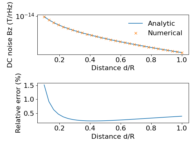
DC magnetic noise from unit disc

mesh = trimesh.load(
    pkg_resources.resource_filename("bfieldtools", "example_meshes/unit_disc.stl")
)
mesh.vertices, mesh.faces = trimesh.remesh.subdivide(mesh.vertices, mesh.faces)
mesh.vertices, mesh.faces = trimesh.remesh.subdivide(mesh.vertices, mesh.faces)

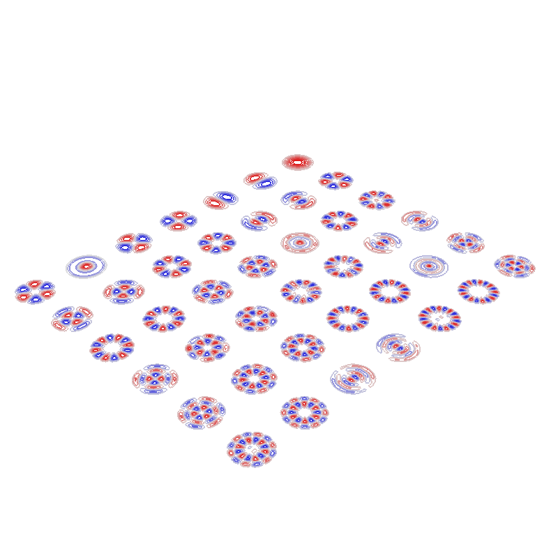
# Compute the AC-current modes and visualize them
vl, u = compute_current_modes(
    obj=mesh, T=T, resistivity=res, thickness=d, mode="AC", return_eigenvals=True
)

scene = mlab.figure(None, bgcolor=(1, 1, 1), fgcolor=(0.5, 0.5, 0.5), size=(800, 800))
visualize_current_modes(mesh, vl[:, :, 0], 42, 5, contours=True)

# Define field points on z axis
Np = 30
z = np.linspace(0.1, 1, Np)
fp = np.array((np.zeros(z.shape), np.zeros(z.shape), z)).T

B_coupling = magnetic_field_coupling(mesh, fp, analytic=True)  # field coupling matrix

# Compute noise variance
B = np.sqrt(noise_var(B_coupling, vl))

# Calculate Bz noise using analytical formula and plot the results
r = 1
Ban = (
    mu0
    * np.sqrt(sigma * d * kB * T / (8 * np.pi * z ** 2))
    * (1 / (1 + z ** 2 / r ** 2))
)

plt.figure()
plt.subplot(2, 1, 1)
plt.semilogy(z, Ban, label="Analytic")
plt.semilogy(z, B[:, 2, 0], "x", label="Numerical")
plt.legend(frameon=False)
plt.xlabel("Distance d/R")
plt.ylabel("DC noise Bz (T/rHz)")

plt.subplot(2, 1, 2)
plt.plot(z, np.abs((B[:, 2, 0] - Ban)) / np.abs(Ban) * 100)
plt.xlabel("Distance d/R")
plt.ylabel("Relative error (%)")
plt.tight_layout()

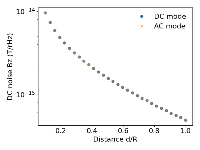
# Next, we compute the DC noise without reference to the inductance
vl_dc, u_dc = compute_current_modes(
    obj=mesh, T=T, resistivity=res, thickness=d, mode="DC", return_eigenvals=True
)

# Compute noise variance
B_dc = np.sqrt(noise_var(B_coupling, vl_dc))

# Compare results computed using AC and DC formulation
plt.figure()
plt.semilogy(z, B_dc[:, 2], "o", label="DC mode")
plt.semilogy(z, B[:, 2, 0], "x", label="AC mode")
plt.legend(frameon=False)
plt.xlabel("Distance d/R")
plt.ylabel("DC noise Bz (T/rHz)")
plt.tight_layout()

• 
• 

Out:

No component count given, computing all components.
Calculating surface harmonics expansion...
Computing the resistance matrix...
Computing the inductance matrix...
Computing self-inductance matrix using rough quadrature (degree=2).              For higher accuracy, set quad_degree to 4 or more.
Estimating 6592 MiB required for 1207 by 1207 vertices...
Computing inductance matrix in 20 chunks (12320 MiB memory free),              when approx_far=True using more chunks is faster...
Computing triangle-coupling matrix
Inductance matrix computation took 2.38 seconds.
0 0
1 0
2 0
3 0
4 0
5 0
6 0
0 1
1 1
2 1
3 1
4 1
5 1
6 1
0 2
1 2
2 2
3 2
4 2
5 2
6 2
0 3
1 3
2 3
3 3
4 3
5 3
6 3
0 4
1 4
2 4
3 4
4 4
5 4
6 4
0 5
1 5
2 5
3 5
4 5
5 5
6 5
Computing magnetic field coupling matrix analytically, 1207 vertices by 30 target points... took 0.05 seconds.
findfont: Font family ['normal'] not found. Falling back to DejaVu Sans.
No component count given, computing all components.
Calculating surface harmonics expansion...
Computing the resistance matrix...
Computing the mass matrix...

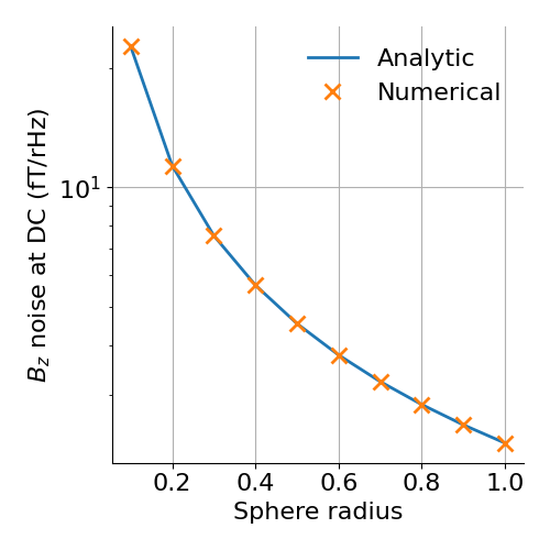
DC magnetic noise in the center of sphere with different radii

Np = 10
radius = np.linspace(0.1, 1, Np)
fp = np.zeros((1, 3))  # calculate are at origin

B = np.zeros((Np, 3))
for i in range(Np):
    mesh = trimesh.load(
        pkg_resources.resource_filename("bfieldtools", "example_meshes/unit_sphere.stl")
    )
    mesh.apply_scale(radius[i])

    B_coupling = magnetic_field_coupling(mesh, fp, analytic=True)

    vl = compute_current_modes(obj=mesh, T=T, resistivity=res, thickness=d, mode="DC")
    Btemp = noise_var(B_coupling, vl)
    B[i] = Btemp

# Analytic formula
Ban = mu0 * np.sqrt(2 * sigma * d * kB * T / (3 * np.pi * (radius) ** 2))

plt.figure(figsize=(5, 5))
plt.semilogy(radius, Ban * 1e15, linewidth=2, label="Analytic")
plt.semilogy(
    radius,
    np.sqrt(B[:, 2]) * 1e15,
    "x",
    markersize=10,
    markeredgewidth=2,
    label="Numerical",
)
plt.grid()
plt.gca().spines["right"].set_visible(False)
plt.gca().spines["top"].set_visible(False)
plt.legend(frameon=False)
plt.xlabel("Sphere radius")
plt.ylabel(r"$B_z$ noise at DC (fT/rHz)")
plt.tight_layout()

Out:

Computing magnetic field coupling matrix analytically, 2562 vertices by 1 target points... took 0.03 seconds.
No component count given, computing all components.
Calculating surface harmonics expansion...
Computing the resistance matrix...
Computing the mass matrix...
Closed mesh or Neumann BC, leaving out the constant component
Computing magnetic field coupling matrix analytically, 2562 vertices by 1 target points... took 0.02 seconds.
No component count given, computing all components.
Calculating surface harmonics expansion...
Computing the resistance matrix...
Computing the mass matrix...
Closed mesh or Neumann BC, leaving out the constant component
Computing magnetic field coupling matrix analytically, 2562 vertices by 1 target points... took 0.02 seconds.
No component count given, computing all components.
Calculating surface harmonics expansion...
Computing the resistance matrix...
Computing the mass matrix...
Closed mesh or Neumann BC, leaving out the constant component
Computing magnetic field coupling matrix analytically, 2562 vertices by 1 target points... took 0.02 seconds.
No component count given, computing all components.
Calculating surface harmonics expansion...
Computing the resistance matrix...
Computing the mass matrix...
Closed mesh or Neumann BC, leaving out the constant component
Computing magnetic field coupling matrix analytically, 2562 vertices by 1 target points... took 0.02 seconds.
No component count given, computing all components.
Calculating surface harmonics expansion...
Computing the resistance matrix...
Computing the mass matrix...
Closed mesh or Neumann BC, leaving out the constant component
Computing magnetic field coupling matrix analytically, 2562 vertices by 1 target points... took 0.02 seconds.
No component count given, computing all components.
Calculating surface harmonics expansion...
Computing the resistance matrix...
Computing the mass matrix...
Closed mesh or Neumann BC, leaving out the constant component
Computing magnetic field coupling matrix analytically, 2562 vertices by 1 target points... took 0.02 seconds.
No component count given, computing all components.
Calculating surface harmonics expansion...
Computing the resistance matrix...
Computing the mass matrix...
Closed mesh or Neumann BC, leaving out the constant component
Computing magnetic field coupling matrix analytically, 2562 vertices by 1 target points... took 0.02 seconds.
No component count given, computing all components.
Calculating surface harmonics expansion...
Computing the resistance matrix...
Computing the mass matrix...
Closed mesh or Neumann BC, leaving out the constant component
Computing magnetic field coupling matrix analytically, 2562 vertices by 1 target points... took 0.02 seconds.
No component count given, computing all components.
Calculating surface harmonics expansion...
Computing the resistance matrix...
Computing the mass matrix...
Closed mesh or Neumann BC, leaving out the constant component
Computing magnetic field coupling matrix analytically, 2562 vertices by 1 target points... took 0.02 seconds.
No component count given, computing all components.
Calculating surface harmonics expansion...
Computing the resistance matrix...
Computing the mass matrix...
Closed mesh or Neumann BC, leaving out the constant component

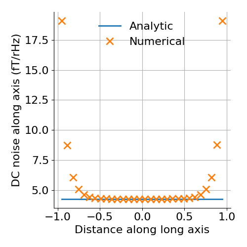
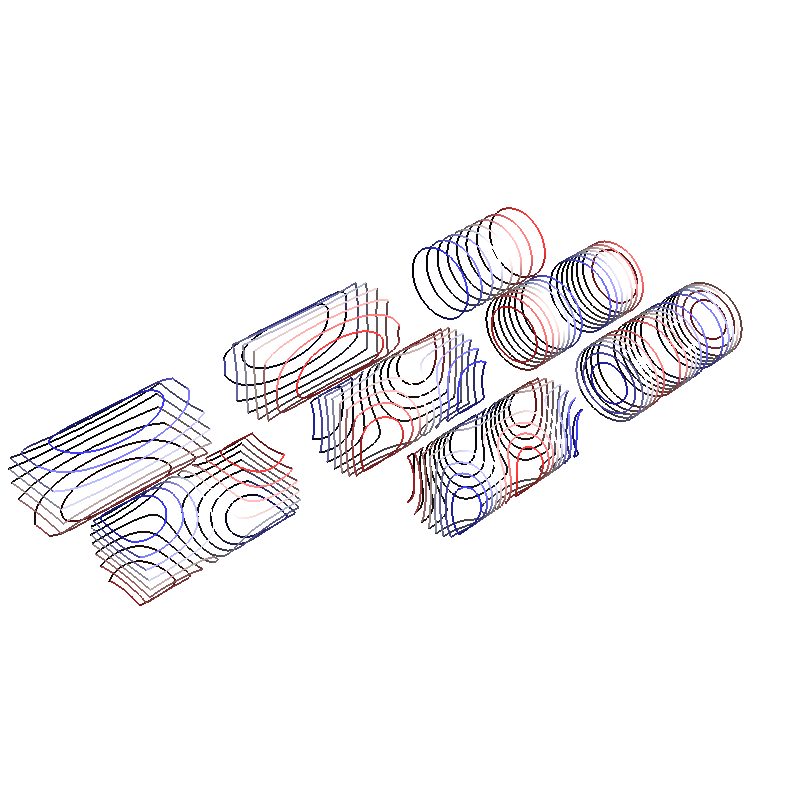
Closed cylinder, DC noise

mesh = trimesh.load(
    pkg_resources.resource_filename("bfieldtools", "example_meshes/closed_cylinder.stl")
)
mesh.vertices, mesh.faces = trimesh.remesh.subdivide(mesh.vertices, mesh.faces)

# Compute noise current modes at DC
vl = compute_current_modes(obj=mesh, T=T, resistivity=res, thickness=d, mode="DC")

# Visualize the current modes
scene = mlab.figure(None, bgcolor=(1, 1, 1), fgcolor=(0.5, 0.5, 0.5), size=(800, 800))
visualize_current_modes(mesh, vl, 8, 1)

# Calculate field noise along long axis of the cylinder
Np = 30
x = np.linspace(-0.95, 0.95, Np)
fp = np.array((x, np.zeros(x.shape), np.zeros(x.shape))).T

B_coupling = magnetic_field_coupling(mesh, fp, analytic=True)
B = noise_var(B_coupling, vl)

# Analytic formula valid only at the center of cylinder
a = 0.5
L = 2
rat = L / (2 * a)
Gfact = (
    1
    / (8 * np.pi)
    * (
        (3 * rat ** 5 + 5 * rat ** 3 + 2) / (rat ** 2 * (1 + rat ** 2) ** 2)
        + 3 * np.arctan(rat)
    )
)
Ban = np.sqrt(Gfact) * mu0 * np.sqrt(kB * T * sigma * d) / a


plt.figure(figsize=(5, 5))
plt.plot(x, Ban * np.ones(x.shape) * 1e15, label="Analytic", linewidth=2)
plt.plot(
    x,
    np.sqrt(B[:, 0]) * 1e15,
    "x",
    label="Numerical",
    markersize=10,
    markeredgewidth=2,
)
plt.grid()
plt.gca().spines["right"].set_visible(False)
plt.gca().spines["top"].set_visible(False)
plt.legend(frameon=False)
plt.xlabel("Distance along long axis")
plt.ylabel("DC noise along axis (fT/rHz)")
plt.tight_layout()

Out:

No component count given, computing all components.
Calculating surface harmonics expansion...
Computing the resistance matrix...
Computing the mass matrix...
Closed mesh or Neumann BC, leaving out the constant component
0 0
1 0
2 0
0 1
1 1
2 1
0 2
1 2
Computing magnetic field coupling matrix analytically, 3842 vertices by 30 target points... took 0.12 seconds.

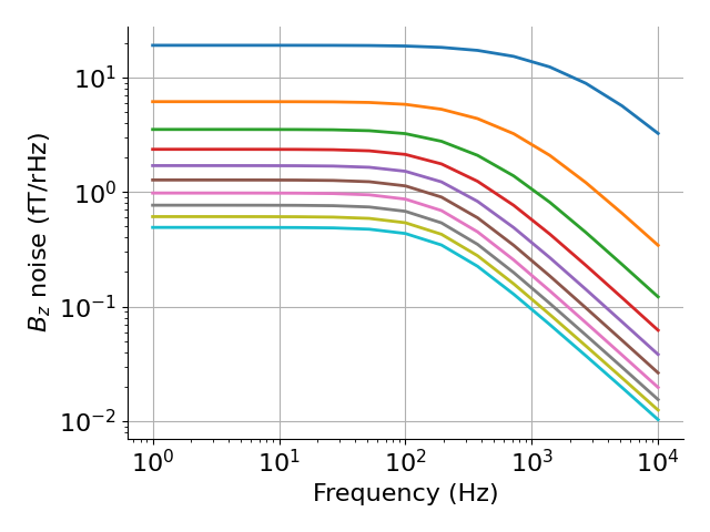
Unit disc, AC noise

mesh = trimesh.load(
    pkg_resources.resource_filename(
        "bfieldtools", "example_meshes/unitdisc_extremelyfine.stl"
    )
)

Nfreqs = 10
freqs = np.logspace(0, 4, 15)  # freqs from 1 to 10 kHz

vl = compute_current_modes(
    obj=mesh,
    T=T,
    resistivity=res,
    thickness=d,
    mode="AC",
    freqs=freqs,
    return_eigenvals=False,
)


Np = 10
z = np.linspace(0.05, 1, Np)
fp = np.array((np.zeros(z.shape), np.zeros(z.shape), z)).T

B_coupling = magnetic_field_coupling(mesh, fp, analytic=True)

Bf = np.sqrt(noise_var(B_coupling, vl))  # noise variance

# Plot Bz noise as a function of frequency
plt.figure()
plt.loglog(freqs, Bf[:, 2, :].T * 1e15, linewidth=2)
plt.grid()
# plt.ylim(1, 20)
plt.gca().spines["right"].set_visible(False)
plt.gca().spines["top"].set_visible(False)
plt.legend(frameon=False)
plt.xlabel("Frequency (Hz)")
plt.ylabel(r"$B_z$ noise (fT/rHz)")
plt.tight_layout()

Out:

No component count given, computing all components.
Calculating surface harmonics expansion...
Computing the resistance matrix...
Computing the inductance matrix...
Computing self-inductance matrix using rough quadrature (degree=2).              For higher accuracy, set quad_degree to 4 or more.
Estimating 27858 MiB required for 2790 by 2790 vertices...
Computing inductance matrix in 60 chunks (11654 MiB memory free),              when approx_far=True using more chunks is faster...
Computing triangle-coupling matrix
Inductance matrix computation took 11.21 seconds.
Computing magnetic field coupling matrix analytically, 2790 vertices by 10 target points... took 0.04 seconds.
No handles with labels found to put in legend.

Estimated memory usage: 1827 MB