Analytic B-field computation

Validation of analytic mesh operator for magnetic field computation.

import numpy as np
import trimesh
from mayavi import mlab
import matplotlib.pyplot as plt

from bfieldtools.mesh_calculus import gradient
from bfieldtools.mesh_magnetics import (
    magnetic_field_coupling,
    magnetic_field_coupling_analytic,
)
from bfieldtools.mesh_conductor import MeshConductor
import pkg_resources


# Load simple plane mesh that is centered on the origin
file_obj = pkg_resources.resource_filename(
    "bfieldtools", "example_meshes/10x10_plane.obj"
)
coilmesh = trimesh.load(file_obj, process=False)
coil = MeshConductor(mesh_obj=coilmesh)
weights = np.zeros(coilmesh.vertices.shape[0])
weights[coil.inner_vertices] = 1

test_points = coilmesh.vertices + np.array([0, 1, 0])

B0 = magnetic_field_coupling(coilmesh, test_points) @ weights
B1 = magnetic_field_coupling_analytic(coilmesh, test_points) @ weights


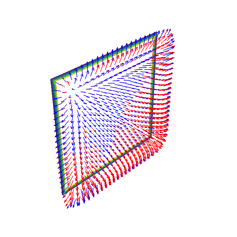
f = mlab.figure(None, bgcolor=(1, 1, 1), fgcolor=(0.5, 0.5, 0.5), size=(800, 800))

s = mlab.triangular_mesh(
    *coilmesh.vertices.T, coilmesh.faces, scalars=weights, colormap="viridis"
)
s.enable_contours = True
s.actor.property.render_lines_as_tubes = True
s.actor.property.line_width = 3.0

mlab.quiver3d(*test_points.T, *B0.T, color=(1, 0, 0))
mlab.quiver3d(*test_points.T, *B1.T, color=(0, 0, 1))

print(
    "Relative RMS error", np.sqrt(np.mean((B1 - B0) ** 2)) / np.sqrt(np.mean((B0) ** 2))
)

Out:

Computing magnetic field coupling matrix, 676 vertices by 676 target points... took 0.12 seconds.
Computing magnetic field coupling matrix analytically, 676 vertices by 676 target points... took 0.48 seconds.
Relative RMS error 0.005229286958362645

Load simple plane mesh that is centered on the origin

file_obj = pkg_resources.resource_filename(
    "bfieldtools", "example_meshes/unit_disc.stl"
)
discmesh = trimesh.load(file_obj, process=True)
for ii in range(3):
    discmesh = discmesh.subdivide()
disc = MeshConductor(mesh_obj=discmesh)
weights = np.zeros(discmesh.vertices.shape[0])
weights[disc.inner_vertices] = 1
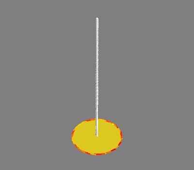
mlab.figure()
s = mlab.triangular_mesh(
    *discmesh.vertices.T, discmesh.faces, scalars=weights, colormap="viridis"
)
g = gradient(weights, discmesh, rotated=True)
mlab.quiver3d(*discmesh.vertices[discmesh.faces].mean(axis=1).T, *g)

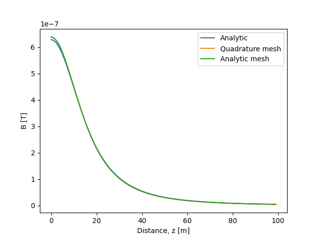
test_points = np.zeros((100, 3))
test_points[:, 2] = np.linspace(0.0, 5, 100)
mlab.points3d(*test_points.T, scale_factor=0.1)

# Bfield for 1 Ampere current
B0 = magnetic_field_coupling(discmesh, test_points) @ weights
B1 = magnetic_field_coupling_analytic(discmesh, test_points) @ weights

# Analytic formula for unit disc
plt.plot(1e-7 * 2 * np.pi / (np.sqrt(test_points[:, 2] ** 2 + 1) ** 3))
# Field from the mesh
plt.plot(np.linalg.norm(B0, axis=1))
plt.plot(np.linalg.norm(B1, axis=1))

plt.legend(("Analytic", "Quadrature mesh", "Analytic mesh"))
plt.xlabel("Distance, z [m]")
plt.ylabel("B [T]")

Out:

Computing magnetic field coupling matrix, 4701 vertices by 100 target points... took 0.30 seconds.
Computing magnetic field coupling matrix analytically, 4701 vertices by 100 target points... took 0.53 seconds.

Text(0, 0.5, 'B [T]')