Linear dipole density on a triangle

Test and validation of potential of linearly distributed dipolar density

For the math see:

J. C. de Munck, “A linear discretization of the volume mesh_conductor boundary integral equation using analytically integrated elements (electrophysiology application),” in IEEE Transactions on Biomedical Engineering, vol. 39, no. 9, pp. 986-990, Sept. 1992. doi: 10.1109/10.256433

import numpy as np
import matplotlib.pyplot as plt
import sys

path = "/m/home/home8/80/makinea1/unix/pythonstuff/bfieldtools"
if path not in sys.path:
    sys.path.insert(0, path)

from bfieldtools.integrals import triangle_potential_dipole_linear
from bfieldtools.integrals import omega
from bfieldtools.utils import tri_normals_and_areas

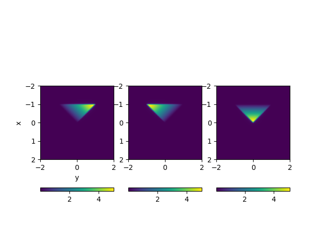
%% Test potential shape slightly above the surface

points = np.array([[0,0,0],

[1,0,0], [0,1,0]])

tris = np.array([[0,1,2]]) p_tris = points[tris]

points = np.array([[0, 0, 0], [1, 1, 0], [1, -1, 0], [-1, -1, 0], [-1, 1, 0]])

tris = np.array([[0, 1, 2], [0, 2, 3], [0, 3, 4], [0, 4, 1]])
tris = np.flip(tris, axis=-1)
p_tris = points[tris]

# Evaluation points
Nx = 100
xx = np.linspace(-2, 2, Nx)
X, Y = np.meshgrid(xx, xx, indexing="ij")
Z = np.zeros_like(X) + 0.01
p_eval = np.array([X, Y, Z]).reshape(3, -1).T

# Difference vectors
RR = p_eval[:, None, None, :] - p_tris[None, :, :, :]
tn, ta = tri_normals_and_areas(points, tris)

pot = triangle_potential_dipole_linear(RR, tn, ta)

# Plot shapes
f, ax = plt.subplots(1, 3)
for i in range(3):
    plt.sca(ax[i])
    plt.imshow(
        pot[:, 2, i].reshape(Nx, Nx), extent=(xx.min(), xx.max(), xx.max(), xx.min())
    )
    plt.colorbar(orientation="horizontal")
    if i == 0:
        plt.ylabel("x")
        plt.xlabel("y")

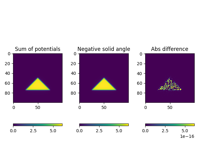
%% Test summation formula

NOTE: the sign of tilde(omega)_i in the bfieldtools (triangle_potential_dipole_linear) is equal to -omega_i in the de Munck’s paper refered above

pot_sum = triangle_potential_dipole_linear(RR, tn, ta).sum(axis=-1)
solid_angle = omega(RR)

# Plot shapes
f, ax = plt.subplots(1, 3)
plt.sca(ax[0])
plt.title("Sum of potentials")
plt.imshow(pot_sum[:, 0].reshape(Nx, Nx), vmin=0, vmax=pot_sum.max())
plt.colorbar(orientation="horizontal")
plt.sca(ax[1])
plt.title("Negative solid angle")
plt.imshow(-solid_angle[:, 0].reshape(Nx, Nx), vmin=0, vmax=pot_sum.max())
plt.colorbar(orientation="horizontal")
plt.sca(ax[2])
plt.title("Abs difference")
plt.imshow(
    abs((-solid_angle[:, 0] - pot_sum[:, 0])).reshape(Nx, Nx),
    vmin=0,
    vmax=pot_sum.max() / 1e16,
)
plt.colorbar(orientation="horizontal", pad=-0.2)
plt.axis("image")

plt.tight_layout()

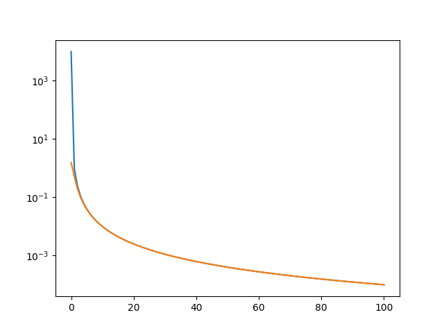
%% Test asymptotic behavour

def dip_potential(Reval, Rdip, moment):
    R = Reval - Rdip
    r = np.linalg.norm(R, axis=1)
    return (moment * R).sum(axis=1) / r ** 3


# Center of mass
Rdip = points.mean(axis=0)
# Moment
m = ta[0] * tn[0]
# Eval points
Neval = 100
p_eval2 = np.zeros((Neval, 3))
z = np.linspace(0.01, 100, Neval)
p_eval2[:, 2] = z
p_eval2 += Rdip


plt.figure()

# Plot dipole field approximating uniform dipolar density
plt.semilogy(z, dip_potential(p_eval2, Rdip, m))
# Plot sum of the linear dipoles
RR = p_eval2[:, None, None, :] - p_tris[None, :, :, :]
pot = triangle_potential_dipole_linear(RR, tn, ta)
plt.semilogy(z, pot.sum(axis=-1)[:, 0])

Out:

[<matplotlib.lines.Line2D object at 0x7f0c11e01e90>]

Estimated memory usage: 9 MB