B-field on the symmetry axis of a disc

Compare a analytic expression and the numerical computation of the B-field of a symmetric current distribution

import numpy as np
import matplotlib.pyplot as plt
import trimesh
from mayavi import mlab
from bfieldtools.mesh_magnetics import magnetic_field_coupling
from bfieldtools.mesh_conductor import MeshConductor, StreamFunction
from bfieldtools.utils import load_example_mesh


def field_disc(z, a):
    """ Bfield z-component of streamfunction psi=r**2 z-axis
        for a disk with radius "a" on the xy plane
    """

    coeff = 1e-7
    field = -2 * (a ** 2 + 2 * z ** 2) / np.sqrt((a ** 2 + z ** 2)) + 4 * abs(z)
    field *= coeff * 2 * np.pi

    return field


# Load disc and subdivide
disc = load_example_mesh("unit_disc")
for i in range(4):
    disc = disc.subdivide()
disc.vertices -= disc.vertices.mean(axis=0)

# Stream functions
s = disc.vertices[:, 0] ** 2 + disc.vertices[:, 1] ** 2

Np = 50
z = np.linspace(-1, 10, Np) + 0.001
points = np.zeros((Np, 3))
points[:, 2] = z
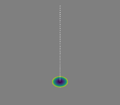
mlab.triangular_mesh(*disc.vertices.T, disc.faces, scalars=s, colormap="viridis")
mlab.points3d(*points.T, scale_factor=0.1)

bfield_mesh = magnetic_field_coupling(disc, points, analytic=True) @ s

Out:

Computing magnetic field coupling matrix analytically, 18553 vertices by 50 target points... took 1.15 seconds.

Nr = 100
drs = np.linspace(-0.0035, -0.0034, Nr)
from matplotlib import cm

colors = cm.viridis(np.linspace(0, 1, Nr))
err = []
for c, dr in zip(colors, drs):
    err.append(
        (abs((bfield_mesh[:, 2] - field_disc(z, 1 + dr)) / field_disc(z, 1 + dr)))[-1]
    )
plt.plot(1 + drs, err)
plt.ylabel("error")
plt.xlabel("disc radius")

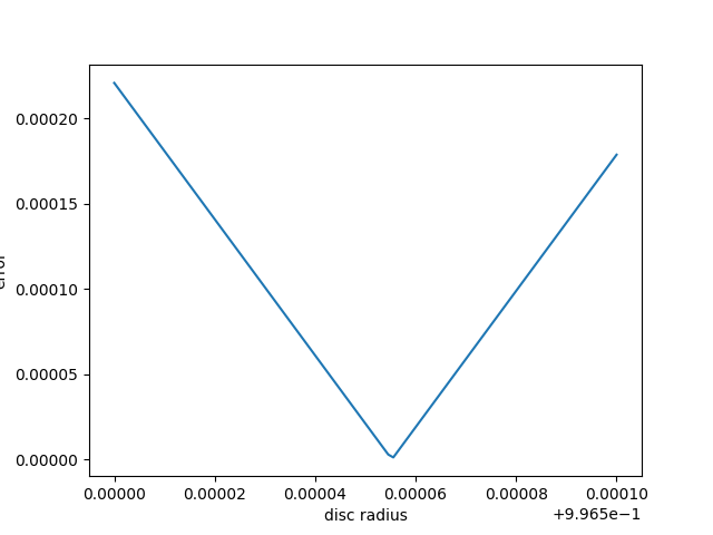
Out:

Text(0.5, 0, 'disc radius')

plt.figure()
# Solve zero-crossing
pp = np.polyfit(drs[:30], err[:30], deg=1)
dr0 = -pp[1] / pp[0]

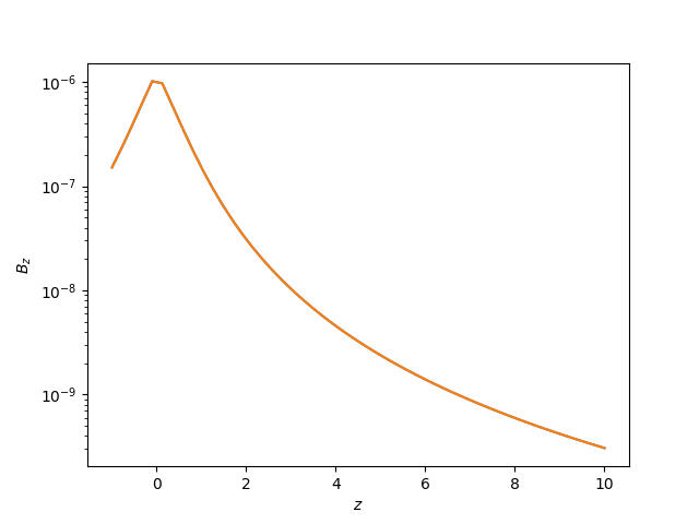
plt.semilogy(z, -field_disc(z, 1 + dr0))
plt.semilogy(z, -bfield_mesh[:, 2])
plt.xlabel("$z$")
plt.ylabel("$B_z$")


plt.figure()
# Plot the relative error
plt.plot(z, (abs(bfield_mesh[:, 2] - field_disc(z, 1 + dr0)) / field_disc(z, 1 + dr0)))
plt.xlabel("$z$")
plt.ylabel("relative error")

• 
• 

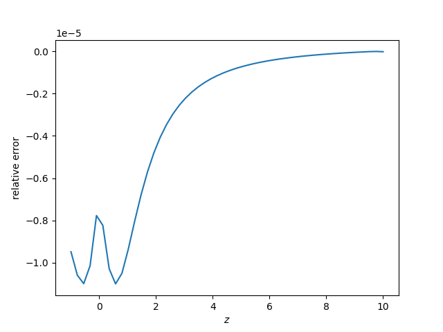
Out:

Text(0, 0.5, 'relative error')

Estimated memory usage: 395 MB