Validate calculation bfield calculation from line segments

import numpy as np
import matplotlib.pyplot as plt
import time as t
from bfieldtools.line_magnetics import magnetic_field

""" Bfield calculation from circular current loops using elliptic integrals
"""


def double_factorial(n):
    if n <= 0:
        return 1
    else:
        return n * double_factorial(n - 2)


def bfield_iterative(x, y, z, x_c, y_c, z_c, r, I, n):
    """ Compute b field of a current loop using an iterative method to estimate
        elliptic integrals.

        Parameters:
            x, y, z: Evaluation points in 3D space. Accepts matrices and integers.
            x_c, y_c, z_c: Coordinates of the center point of the current loop.
            r: Radius of the current loop.
            I: Current of the current loop.
            n: Number of terms in the serie expansion.

        Returns:
            bfiels (N_points, 3) at evaluation points.

        This calculation is based on paper by Robert A. Schill, Jr (General
        Relation for the Vector Magnetic Field of aCircular Current Loop:
        A Closer Look). DOI: 10.1109/TMAG.2003.808597
    """

    st2 = t.time()
    np.seterr(divide="ignore", invalid="ignore")
    u0 = 4 * np.pi * 1e-7
    Y = u0 * I / (2 * np.pi)

    # Change to cylideric coordinates
    rc = np.sqrt(np.power(x - x_c, 2) + np.power(y - y_c, 2))

    # Coefficients for estimating elliptic integrals with nth degree series
    # expansion using Legendre polynomials
    m = 4 * r * rc / (np.power((rc + r), 2) + np.power((z - z_c), 2))
    K = 1
    E = 1
    for i in range(1, n + 1):
        K = K + np.square(
            double_factorial(2 * i - 1) / double_factorial(2 * i)
        ) * np.power(m, i)
        E = E - np.square(
            double_factorial(2 * i - 1) / double_factorial(2 * i)
        ) * np.power(m, i) / (2 * i - 1)

    K = K * np.pi / 2
    E = E * np.pi / 2

    # Calculation of radial and axial components of B-field
    Brc = (
        Y
        * (z - z_c)
        / (rc * np.sqrt(np.power((rc + r), 2) + np.power((z - z_c), 2)))
        * (
            -K
            + E
            * (np.power(rc, 2) + np.power(r, 2) + np.power((z - z_c), 2))
            / (np.power((rc - r), 2) + np.power((z - z_c), 2))
        )
    )

    Bz = (
        Y
        / (np.sqrt(np.power((rc + r), 2) + np.power((z - z_c), 2)))
        * (
            K
            - E
            * (np.power(rc, 2) - np.power(r, 2) + np.power((z - z_c), 2))
            / (np.power((rc - r), 2) + np.power((z - z_c), 2))
        )
    )

    # Set nan and inf values to 0
    Brc[np.isinf(Brc)] = 0
    Bz[np.isnan(Bz)] = 0
    Brc[np.isnan(Brc)] = 0
    Bz[np.isinf(Bz)] = 0

    # Change back to cartesian coordinates
    Bx = Brc * (x - x_c) / rc
    By = Brc * (y - y_c) / rc

    # Change nan values from coordinate transfer to 0
    Bx[np.isnan(Bx)] = 0
    By[np.isnan(By)] = 0

    B = np.zeros((3, X.size), dtype=np.float64)
    B[0] = Bx.flatten()
    B[1] = By.flatten()
    B[2] = Bz.flatten()

    et2 = t.time()
    print("Execution time for iterative method is:", et2 - st2)

    return B.T


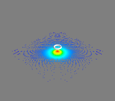
""" Plot field of a circular current path
"""
x = np.linspace(-1, 1, 100)
Ntheta = 10000
theta = np.linspace(0, 2 * np.pi, Ntheta)
vertices = np.zeros((Ntheta, 3), dtype=np.float64)
vertices[:, 0] = np.cos(theta) * 0.1
vertices[:, 1] = np.sin(theta) * 0.1
vertices[:, 2] = 0.2

X, Y = np.meshgrid(x, x, indexing="ij")
Z = np.zeros((x.size, x.size))

points = np.zeros((3, X.size), dtype=np.float64)
points[0] = X.flatten()
points[1] = Y.flatten()

b1 = magnetic_field(vertices, points.T)  # Calculates discretised bfield
b2 = bfield_iterative(X, Y, Z, 0, 0, 0.2, 0.1, 1, 25)  # Calculates bfield iteratively

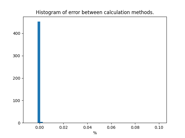
# Error between two calculation methods.
berr = (b2 - b1) / b1 * 100
BE = berr.T[2]  # By changing the index, errors in different components can be obtained
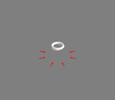
ind = np.where(np.abs(BE) > 0.1)  # The limit for significant error is set to 0.1%
bpoints = points.T[ind]

from mayavi import mlab

mlab.figure(1)
q = mlab.quiver3d(*points, *b1.T)
q.glyph.glyph_source.glyph_position = "center"
mlab.plot3d(*vertices.T)

mlab.figure(2)
q = mlab.quiver3d(*points, *b2.T)
q.glyph.glyph_source.glyph_position = "center"
mlab.plot3d(*vertices.T)

plt.figure(3)
plt.hist(berr.T[2], bins=50, density=True, histtype="bar")
plt.title("Histogram of error between calculation methods.")
plt.xlabel("%")

• 
• 

Out:

Execution time for iterative method is: 0.01274728775024414

Text(0.5, 0, '%')

if len(bpoints > 0):

    from mayavi import mlab

    mlab.figure(3)
    q = mlab.quiver3d(*bpoints.T, *b1[ind].T)
    q.glyph.glyph_source.glyph_position = "center"
    mlab.plot3d(*vertices.T)

    q = mlab.quiver3d(*bpoints.T, *b2[ind].T)
    q.glyph.glyph_source.glyph_position = "center"