Validation of self inductance using spherical harmonics

Study the eigenvalue spectrum of the discretize self-inductance operator on a spherical mesh. Compare the spectrum to analytical solution

import numpy as np
from bfieldtools.mesh_impedance import self_inductance_matrix, mutual_inductance_matrix
from bfieldtools.mesh_calculus import mass_matrix
from bfieldtools.utils import load_example_mesh
from scipy.linalg import eigh
import matplotlib.pyplot as plt
import trimesh

# This is icosphere(4)?
# mesh = load_example_mesh("unit_sphere")
# The test is faster with a smaller number of vertices
mesh = trimesh.creation.icosphere(3)

Nvals = 150
uu1 = []
uu2 = []
vv1 = []
vv2 = []
M = mass_matrix(mesh)

for q in range(4):
    L = self_inductance_matrix(mesh, analytic_self_coupling=True, quad_degree=q + 1)
    uu, vv = eigh(L, M.toarray(), eigvals=(0, Nvals - 1))
    uu1.append(uu)
    vv1.append(vv)

    # L = self_inductance_matrix(mesh, analytic_self_coupling=False,
    # quad_degree=q+1)
    L = mutual_inductance_matrix(mesh, mesh, quad_degree=q + 1)
    uu, vv = eigh(L, M.toarray(), eigvals=(0, Nvals - 1))
    uu2.append(uu)
    vv2.append(vv)

Out:

Computing self-inductance matrix using rough quadrature (degree=1).              For higher accuracy, set quad_degree to 4 or more.
Estimating 2225 MiB required for 642 by 642 vertices...
Computing inductance matrix in 20 chunks (10556 MiB memory free),              when approx_far=True using more chunks is faster...
Computing triangle-coupling matrix
Estimating 2225 MiB required for 642 by 642 vertices...
Computing inductance matrix in 20 chunks (10557 MiB memory free),              when approx_far=True using more chunks is faster...
Computing triangle-coupling matrix
Computing self-inductance matrix using rough quadrature (degree=2).              For higher accuracy, set quad_degree to 4 or more.
Estimating 2225 MiB required for 642 by 642 vertices...
Computing inductance matrix in 20 chunks (10557 MiB memory free),              when approx_far=True using more chunks is faster...
Computing triangle-coupling matrix
Estimating 2225 MiB required for 642 by 642 vertices...
Computing inductance matrix in 20 chunks (10558 MiB memory free),              when approx_far=True using more chunks is faster...
Computing triangle-coupling matrix
Estimating 2225 MiB required for 642 by 642 vertices...
Computing inductance matrix in 20 chunks (10556 MiB memory free),              when approx_far=True using more chunks is faster...
Computing triangle-coupling matrix
Estimating 2225 MiB required for 642 by 642 vertices...
Computing inductance matrix in 20 chunks (10556 MiB memory free),              when approx_far=True using more chunks is faster...
Computing triangle-coupling matrix
Estimating 2225 MiB required for 642 by 642 vertices...
Computing inductance matrix in 20 chunks (10544 MiB memory free),              when approx_far=True using more chunks is faster...
Computing triangle-coupling matrix
Estimating 2225 MiB required for 642 by 642 vertices...
Computing inductance matrix in 20 chunks (10544 MiB memory free),              when approx_far=True using more chunks is faster...
Computing triangle-coupling matrix

"""
 Spherical harmonics are the eigenfunctions of self-inductance operator
 The correct eigenvalues derived using Taulu 2005 Eqs. (22, 23, A1, A5, A6)
 By considering the normal component of the magnetic field produced by
 a single Y_lm. The result is
 e = mu_0*(l*(l+1)/(2*l+1))/R
"""
R = np.linalg.norm(mesh.vertices[mesh.faces].mean(axis=1), axis=-1).mean()
mu0 = (1e-7) * 4 * np.pi
ll = np.array([l for l in range(20) for m in range(-l, l + 1)])
ll = ll[:Nvals]
evals = ll * (ll + 1) / (2 * ll + 1)

plt.plot(evals, ‘k’)

for u in uu1:
    uu_scaled = u / mu0 * R
    plt.plot(abs(evals[1:] - uu_scaled[1:]) / evals[1:], "-")
    # plt.plot(uu_scaled)
plt.legend(("qd=1", "qd=2", "qd=3", "qd=4"))
plt.gca().set_prop_cycle(None)
for u in uu2:
    uu_scaled = u / mu0 * R
    plt.plot(abs(evals[1:] - uu_scaled[1:]) / evals[1:], "--")
plt.title("solid using self_inductance, dashed using mutual_inductance")
plt.xlabel("# eigenvalue")
plt.ylabel("Relative error")

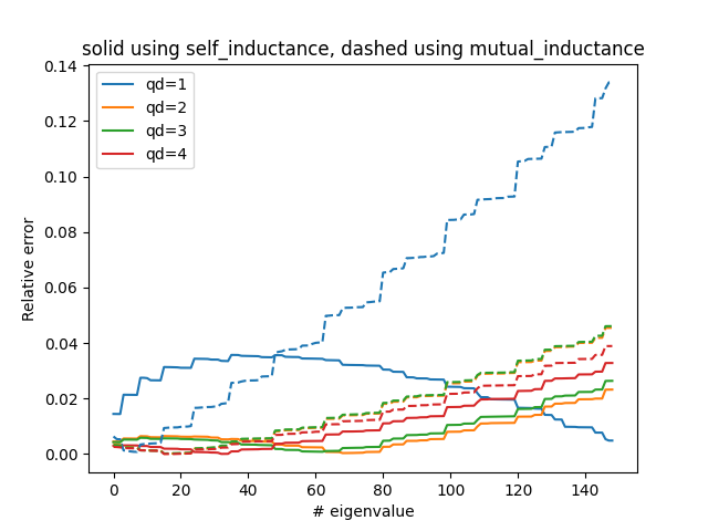
Out:

Text(0, 0.5, 'Relative error')

from bfieldtools.utils import MeshProjection
from bfieldtools.sphtools import ylm
from bfieldtools.sphtools import cartesian2spherical

ylm_on_hats = []
i1 = 0
vv1_projs = np.zeros((len(vv1), vv1[0].shape[1]))
vv2_projs = np.zeros((len(vv2), vv2[0].shape[1]))
mp = MeshProjection(mesh, 4)


for l in range(0, 13):
    i0 = i1
    print(f"l={l}")
    for m in range(-l, l + 1):

        def func(r):
            sphcoords = cartesian2spherical(r)
            return ylm(l, m, sphcoords[:, 1], sphcoords[:, 2])

        ylm_on_hats.append(mp.hatfunc_innerproducts(func))
        i1 += 1
    for ii, vv in enumerate(vv1):
        # Project self-inductance eigenfunctions to l-subspace
        p = np.sum((np.array(ylm_on_hats[i0:i1]) @ vv[:, i0:i1]) ** 2, axis=0)
        vv1_projs[ii, i0:i1] = p
    for ii, vv in enumerate(vv2):
        # Project self-inductance eigenfunctions to l-subspace
        p = np.sum((np.array(ylm_on_hats[i0:i1]) @ vv[:, i0:i1]) ** 2, axis=0)
        vv2_projs[ii, i0:i1] = p

Out:

l=0
l=1
l=2
l=3
l=4
l=5
l=6
l=7
l=8
l=9
l=10
l=11
l=12

plt.figure()
eff_R2 = 1  # np.sum(mesh.area_faces) / (4 * np.pi)
plt.plot(vv1_projs.T / eff_R2, "-")
plt.legend(("qd=1", "qd=2", "qd=3", "qd=4"))
plt.gca().set_prop_cycle(None)
plt.plot(vv2_projs.T / eff_R2, "--")
plt.title("solid using self_inductance, dashed using mutual_inductance")

plt.xlabel("# eigenfunction")
plt.ylabel("Squared norm in L-subspace")

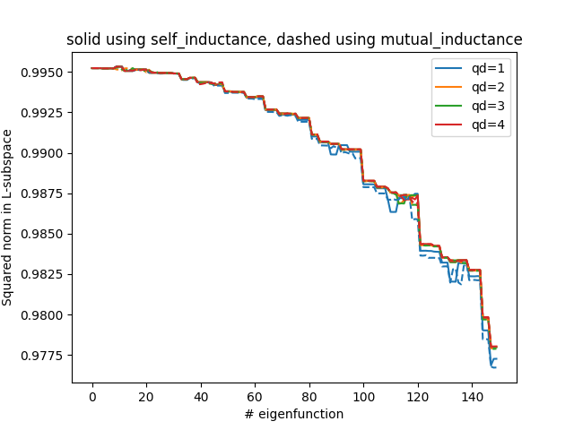
Out:

Text(0, 0.5, 'Squared norm in L-subspace')