One-element fields

import numpy as np

from bfieldtools.mesh_magnetics import (
    scalar_potential_coupling,
    vector_potential_coupling,
)
from bfieldtools.mesh_magnetics import (
    magnetic_field_coupling,
    magnetic_field_coupling_analytic,
)

import trimesh
from mayavi import mlab

# Define the element
x = np.sin(np.pi / 6)
y = np.cos(np.pi / 6)
points0 = np.array(
    [[0, 0, 0], [1, 0, 0], [x, y, 0], [-x, y, 0], [-1, 0, 0], [-x, -y, 0], [x, -y, 0]]
)

tris0 = np.array([[0, 1, 2], [0, 2, 3], [0, 3, 4], [0, 4, 5], [0, 5, 6], [0, 6, 1]])
mesh = trimesh.Trimesh(points0, tris0)
scalars = np.zeros(7)
scalars[0] = 1

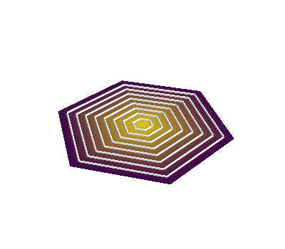
%% Plot element

def plot_element():
    # Stream function
    s1 = mlab.triangular_mesh(*points0.T, tris0, scalars=scalars, colormap="viridis")
    # Stream lines
    s2 = mlab.triangular_mesh(*points0.T, tris0, scalars=scalars, colormap="viridis")
    s2.enable_contours = True
    s2.actor.mapper.scalar_range = np.array([0.0, 1.0])
    s2.actor.mapper.scalar_visibility = False
    s2.actor.property.render_lines_as_tubes = True
    s2.actor.property.line_width = 3.0


mlab.figure(bgcolor=(1, 1, 1))
plot_element()

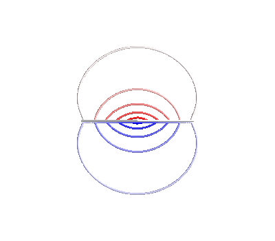
%% Scalar potential

points = np.array([[0.01, 1, 1], [0.01, 1, -1], [0.01, -1, -1], [0.01, -1, 1]]) * 2
tris = np.array([[0, 1, 2], [2, 3, 0]])
mesh2 = trimesh.Trimesh(points, tris)
for ii in range(7):
    mesh2 = mesh2.subdivide()

U = scalar_potential_coupling(mesh, mesh2.vertices, multiply_coeff=True) @ scalars
mlab.figure(bgcolor=(1, 1, 1))
s3 = mlab.triangular_mesh(*mesh2.vertices.T, mesh2.faces, scalars=U, colormap="bwr")
s3.enable_contours = True
s3.contour.minimum_contour = -5.2e-07
s3.contour.maximum_contour = 5.2e-07
s3.actor.property.render_lines_as_tubes = True
s3.actor.property.line_width = 3.0
s3.scene.x_plus_view()
plot_element()

Out:

Computing scalar potential coupling matrix, 7 vertices by 16641 target points... took 0.33 seconds.

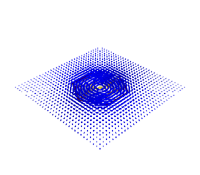
%% Vector potential

points = np.array([[1, 1, 0.01], [1, -1, 0.01], [-1, -1, 0.01], [-1, 1, 0.01]]) * 2
tris = np.array([[0, 1, 2], [2, 3, 0]])
mesh3 = trimesh.Trimesh(points, tris)
for ii in range(5):
    mesh3 = mesh3.subdivide()
A = vector_potential_coupling(mesh, mesh3.vertices) @ scalars
mlab.figure(bgcolor=(1, 1, 1))
vectors = mlab.quiver3d(*mesh3.vertices.T, *A, mode="2ddash", color=(0, 0, 1))
vectors.glyph.glyph_source.glyph_position = "center"
vectors.actor.property.render_lines_as_tubes = True
vectors.actor.property.line_width = 3.0
plot_element()

Out:

Computing triangle-coupling matrix

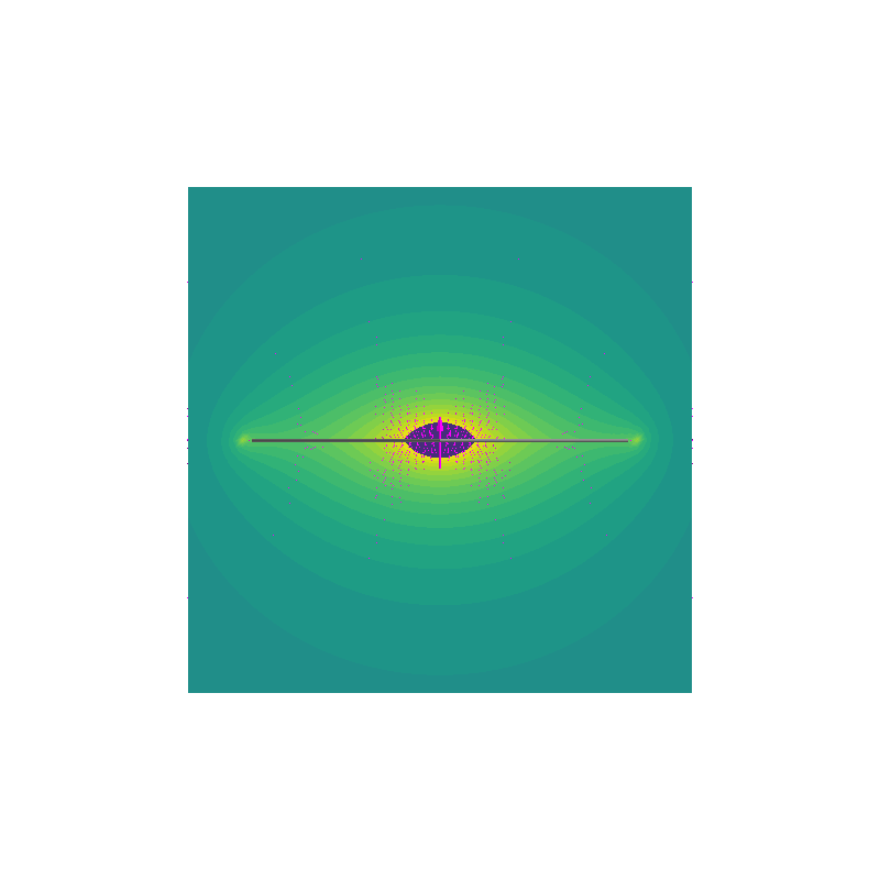
%% Magnetic field and its magnitude

from bfieldtools.viz import plot_data_on_vertices

points = (
    np.array([[0.0, 1, 1.001], [0.0, 1, -1], [0.0, -1, -1], [0.0, -1, 1.001]]) * 1.1
)
tris = np.array([[0, 1, 2], [2, 3, 0]])
mesh2 = trimesh.Trimesh(points, tris)
for ii in range(6):
    mesh2 = mesh2.subdivide()

# B0 = magnetic_field_coupling(mesh, mesh2.vertices) @ scalars
B1 = magnetic_field_coupling_analytic(mesh, mesh2.vertices) @ scalars
plot_data_on_vertices(
    mesh2, np.linalg.norm(B1, axis=1), ncolors=32, colormap="viridis", vmax=1.5e-6
)
vectors = mlab.quiver3d(
    *mesh2.vertices.T, *B1.T, mode="arrow", color=(1, 0, 1), scale_factor=5e4
)
vectors.glyph.glyph_source.glyph_position = "center"
# vectors = mlab.quiver3d(*mesh2.vertices.T, *B0.T, mode="arrow", color=(1, 0, 0))
# vectors.glyph.glyph_source.glyph_position = "center"
plot_element()
vectors.scene.x_plus_view()

Out:

Computing magnetic field coupling matrix analytically, 7 vertices by 4225 target points... took 0.04 seconds.

Estimated memory usage: 136 MB