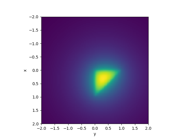
Uniform triangle

Test and validation of potential of uniformaly distributed charge density

For the math see:

A. S. Ferguson, Xu Zhang and G. Stroink, “A complete linear discretization for calculating the magnetic field using the boundary element method,” in IEEE Transactions on Biomedical Engineering, vol. 41, no. 5, pp. 455-460, May 1994. doi: 10.1109/10.293220

import numpy as np
import matplotlib.pyplot as plt
import sys
from mayavi import mlab

path = "/m/home/home8/80/makinea1/unix/pythonstuff/bfieldtools"
if path not in sys.path:
    sys.path.insert(0, path)

from bfieldtools.integrals import triangle_potential_uniform
from bfieldtools.utils import tri_normals_and_areas

%% Test potential shape slightly above the surface

points = np.array([[0, 0, 0], [1, 0, 0], [0, 1, 0]])

tris = np.array([[0, 1, 2]])
p_tris = points[tris]

# Evaluation points
Nx = 100
xx = np.linspace(-2, 2, Nx)
X, Y = np.meshgrid(xx, xx, indexing="ij")
Z = np.zeros_like(X) + 0.01
p_eval = np.array([X, Y, Z]).reshape(3, -1).T

# Difference vectors
RR = p_eval[:, None, None, :] - p_tris[None, :, :, :]
tn, ta = tri_normals_and_areas(points, tris)

pot = triangle_potential_uniform(RR, tn, False)

# Plot shape
plt.figure()
plt.imshow(pot[:, 0].reshape(Nx, Nx), extent=(xx.min(), xx.max(), xx.max(), xx.min()))
plt.ylabel("x")
plt.xlabel("y")

Out:

Text(0.5, 0, 'y')

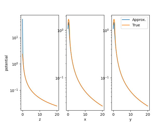
%% Test asymptotic behavour by comparing potential of charge at the

center of mass of the triangle having the same first moment

def charge_potential(Reval, Rcharge, moment):
    R = Reval - Rcharge
    r = np.linalg.norm(R, axis=1)
    return moment / r


# Center of mass
Rcharge = points.mean(axis=0)
# Moment
m = ta
# Eval points
Neval = 100

cases = np.arange(3)
f, ax = plt.subplots(1, 3)
mlab.figure(bgcolor=(1, 1, 1))
mlab.triangular_mesh(*points.T, tris, color=(0.5, 0.5, 0.5))
for c in cases:
    p_eval2 = np.zeros((Neval, 3))

    if c == 0:
        z = np.linspace(0.01, 20, Neval)
        p_eval2[:, 2] = z
        p_eval2 += Rcharge
        mlab.points3d(*p_eval2.T, color=(1, 0, 0), scale_factor=0.1)
        lab = "z"
    elif c == 1:
        x = np.linspace(0.01, 20, Neval)
        p_eval2[:, 0] = x
        mlab.points3d(*p_eval2.T, color=(0, 1, 0), scale_factor=0.1)
        lab = "x"
    elif c == 2:
        y = np.linspace(0.01, 20, Neval)
        p_eval2[:, 1] = y
        mlab.points3d(*p_eval2.T, color=(0, 0, 1), scale_factor=0.1)
        lab = "y"

    plt.sca(ax[c])
    # Plot dipole field approximating uniform dipolar density
    plt.semilogy(z, charge_potential(p_eval2, Rcharge, m))
    # Plot sum of the linear dipoles
    RR = p_eval2[:, None, None, :] - p_tris[None, :, :, :]
    pot = triangle_potential_uniform(RR, tn, False)
    plt.semilogy(z, pot)
    plt.xlabel(lab)
    if c == 0:
        plt.ylabel("potential")
    if c == 2:
        plt.legend(("Approx.", "True"))

Estimated memory usage: 9 MB