Line charge

Test and validation of gamma_0

For the math see:

A. S. Ferguson, Xu Zhang and G. Stroink, “A complete linear discretization for calculating the magnetic field using the boundary element method,” in IEEE Transactions on Biomedical Engineering, vol. 41, no. 5, pp. 455-460, May 1994. doi: 10.1109/10.293220

import pyvista as pv

pv.set_plot_theme("document")


import numpy as np
import matplotlib.pyplot as plt
import sys

path = "/m/home/home8/80/makinea1/unix/pythonstuff/bfieldtools"
if path not in sys.path:
    sys.path.insert(0, path)

from bfieldtools.integrals import gamma0
from bfieldtools.utils import tri_normals_and_areas

%% Test potential shape slightly above the surface

points = np.array([[0, 0, 0], [1, 0, 0], [0, 1, 0]])

tris = np.array([[0, 1, 2]])
p_tris = points[tris]

# Evaluation points
Nx = 100
xx = np.linspace(-2, 2, Nx)
X, Y = np.meshgrid(xx, xx, indexing="ij")
Z = np.zeros_like(X) + 0.1
p_eval = np.array([X, Y, Z]).reshape(3, -1).T

# Difference vectors
RR = p_eval[:, None, None, :] - p_tris[None, :, :, :]

pot = gamma0(RR)

# Plot shape
plt.figure()
plt.imshow(
    pot[:, 0].sum(axis=-1).reshape(Nx, Nx),
    extent=(xx.min(), xx.max(), xx.max(), xx.min()),
)
plt.ylabel("x")
plt.xlabel("y")

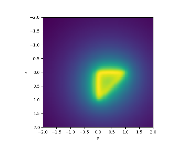
Text(0.5, 23.633333333333333, 'y')

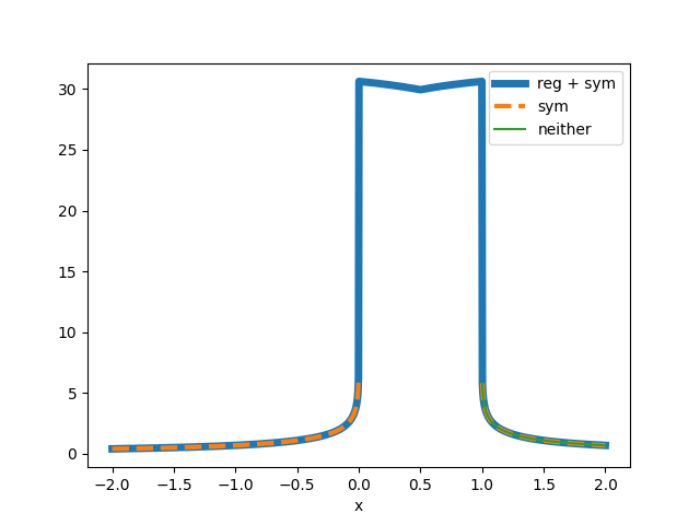
""" Test potential at directly at the edge. As the line has no
    perpendicular dimensions, the potential is infinite at the edge.
    The regularization factor given to the function apprximates the line
    current with a small radius, giving rougly constant potential on the line.
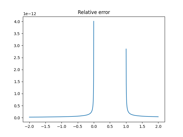
    The relative error between the regularized verison and
    the infinitely thin line charge seems to be on the order of the "reg" value

    The "symmetrize" option symmeterizes the result with respect to the
    mid point. This removes errors (Nans) on the other continuoation of the edge
"""

' Test potential at directly at the edge. As the line has no\n    perpendicular dimensions, the potential is infinite at the edge.\n    The regularization factor given to the function apprximates the line\n    current with a small radius, giving rougly constant potential on the line.\n    The relative error between the regularized verison and\n    the infinitely thin line charge seems to be on the order of the "reg" value\n\n    The "symmetrize" option symmeterizes the result with respect to the\n    mid point. This removes errors (Nans) on the other continuoation of the edge\n'

points = np.array([[0, 0, 0], [1, 0, 0], [0, 1, 0]])

tris = np.array([[0, 1, 2]])
p_tris = points[tris]

# Evaluation points
Nx = 1000
x = np.linspace(-2, 2, Nx)
y = z = np.zeros_like(x)
p_eval = np.array([x, y, z]).T

# Difference vectors
RR = p_eval[:, None, None, :] - p_tris[None, :, :, :]

# Regularize and symmetrize
pot = gamma0(RR, 1e-13, True)
pot0 = pot[:, 0, 2]
plt.figure()
plt.plot(x, pot0, linewidth=5)
# Symmetrize, but do not regularize
pot = gamma0(RR, 0, True)
pot1 = pot[:, 0, 2]
plt.plot(x, pot1, "--", linewidth=3)
# Neither
pot = gamma0(RR, 0, False)
pot2 = pot[:, 0, 2]
plt.plot(x, pot2)
plt.xlabel("x")
plt.legend(("reg + sym", "sym", "neither"))

plt.figure()
plt.title("Relative error")
plt.plot(x, abs(pot0 - pot1) / pot1)

# Display the assembled scene (Sphinx-Gallery captures it during docs builds).
if "plotter" in globals() and not plotter._closed:
    plotter.show()

• 
• 

/home/runner/work/bfieldtools.github.io/bfieldtools.github.io/bfieldtools/integrals.py:82: RuntimeWarning: invalid value encountered in divide
  res = np.log((nn1 + dotprods1 + reg) / (nn2 + dotprods2 + reg))
/home/runner/work/bfieldtools.github.io/bfieldtools.github.io/bfieldtools/integrals.py:82: RuntimeWarning: divide by zero encountered in log
  res = np.log((nn1 + dotprods1 + reg) / (nn2 + dotprods2 + reg))
/home/runner/work/bfieldtools.github.io/bfieldtools.github.io/bfieldtools/integrals.py:90: RuntimeWarning: divide by zero encountered in divide
  (nn1[mask] - dotprods1[mask] + reg) / (nn2[mask] - dotprods2[mask] + reg)
/home/runner/work/bfieldtools.github.io/bfieldtools.github.io/examples/validation/validate_line_charge_potential.py:105: RuntimeWarning: invalid value encountered in divide
  plt.plot(x, abs(pot0 - pot1) / pot1)