Current loop inside a cylindrical magnetic shield

This example calculates the magnetic field produced by a rectangular current loop inside a cylindrical magnetic shield.

import pyvista as pv
from bfieldtools._example_plots import triangle_mesh, polyline, set_view

pv.set_plot_theme("document")


import matplotlib.pyplot as plt
import numpy as np

from bfieldtools.line_magnetics import magnetic_field
from bfieldtools.line_magnetics import scalar_potential
from bfieldtools.mesh_conductor import MeshConductor
from bfieldtools.mesh_conductor import StreamFunction
from bfieldtools.utils import load_example_mesh


def create_3d_grid(xx, yy, zz):
    """Creates a direct product grid from three 1D arrays (xx, yy and zz)
    that is appropriately formated for `scalar_potential` and `magnetic_field`.
    """
    X, Y, Z = np.meshgrid(xx, yy, zz, indexing="ij")

    x = X.ravel()
    y = Y.ravel()
    z = Z.ravel()

    return np.array([x, y, z]).T


# Defines a rectangular current loop offset by y from the xz plane
length = 0.3  # (m)
width = 6e-2  # (m)
ly = 6e-2  # (m)
loop_points = np.array(
    [
        [width / 2, ly, length / 2],
        [width / 2, ly, -length / 2],
        [-width / 2, ly, -length / 2],
        [-width / 2, ly, length / 2],
        [width / 2, ly, length / 2],
    ]
)


# Loads the cylinder shield geometry from examples
shield_mesh = load_example_mesh("closed_cylinder_remeshed")

# Shrinks the shield and rotates it by 90 degrees around the y axis.
shield_mesh.apply_scale(0.17)
shield_mesh.apply_transform([[0, 0, 1, 0], [0, 1, 0, 0], [1, 0, 0, 0], [0, 0, 0, 0]])

shield = MeshConductor(
    mesh_obj=shield_mesh, process=True, fix_normals=True, basis_name="vertex"
)

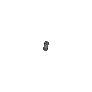
# Plots the complete geometry.
plotter = f1 = pv.Plotter(window_size=(300, 300))
set_view(f1, roll=45, azimuth=50, elevation=60)
f1.add_mesh(polyline(*loop_points.T).tube(radius=0.001), show_scalar_bar=False)
f1.add_mesh(
    triangle_mesh(*shield_mesh.vertices.T, shield_mesh.faces),
    color=(0, 0, 0),
    opacity=0.05,
    style="wireframe",
    show_scalar_bar=False,
)


# Calculates the stream function on the surface of the shield
shield = MeshConductor(mesh_obj=shield_mesh, process=True, fix_normals=True)

# In the following, we want to calculate scalar potentials on the surface of
# the shield. Since the potential created by the surface shield currents is
# discontinuous on the shield, we select the inner surface by taking a small
# offset along the inner normal.
d = 1e-5
shield_inner_points = shield_mesh.vertices - d * shield_mesh.vertex_normals

# Calculates the coupling matrix that relates the stream function of currents
# of the surface of the shield to scalar potential.
U_cpl_ssurf = shield.U_coupling(shield_inner_points)

# Takes the scalar potential created by the current loop at the shield and finds
# the stream function of surface currents that is necessary to compensate it.
U_loop_ssurf = scalar_potential(loop_points, shield_inner_points)
I_shield = np.linalg.solve(-U_cpl_ssurf, U_loop_ssurf)

# Represent the stream function using a dedicated class for visualization.
s_shield = StreamFunction(I_shield, shield)

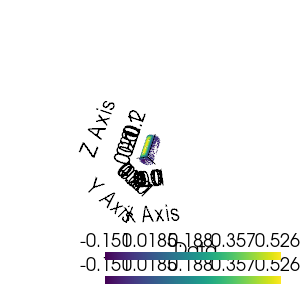
# Visualizes the stream function on the shield.
plotter = f3 = pv.Plotter(window_size=(300, 300))
set_view(f3, roll=45, azimuth=45, elevation=60)
plotter = s_shield.plot(False, 64, figure=f3)
plotter.add_scalar_bar()
plotter.show_bounds()

Static Scene

Interactive Scene

Static Scene

Interactive Scene

Computing scalar potential coupling matrix, 2773 vertices by 2773 target points... took 7.35 seconds.

<CubeAxesActor(0x559797747420) at 0x7f1298fe3e80>

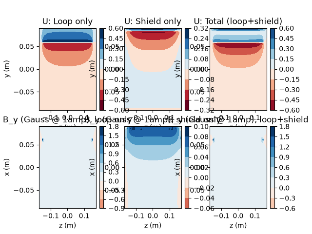
The rest of the code calculates magnetic field on a 2D grid and displays the contributions of the current loop and the shield.

# Defines a grid in the yz plane.
x0 = 0
ny = 50
nz = 100

xx = np.linspace(x0, x0, 1)
yy = np.linspace(-0.9e-1, 0.9e-1, ny)
zz = np.linspace(-0.34 / 2, 0.34 / 2, nz)

grid = create_3d_grid(xx, yy, zz)


# Finds the scalar potential produced by the loop in the absence of shield.
U_loop1 = scalar_potential(loop_points, grid)
U_loop_pl1 = U_loop1.reshape(ny, nz)  # Reshapes for plotting.

# Finds the potential created by the shield.
U_cpl_shield1 = shield.U_coupling(grid)
U_shield1 = U_cpl_shield1 @ I_shield
U_shield_pl1 = U_shield1.reshape(ny, nz)  # Reshapes for plotting.

Computing scalar potential coupling matrix, 2773 vertices by 5000 target points... took 13.08 seconds.

fig, axs = plt.subplots(2, 3)

plt.sca(axs[0, 0])
vmax = np.max(np.abs(U_loop1))
plt.contourf(zz, yy, U_loop_pl1, cmap=plt.get_cmap("RdBu"), vmax=vmax, vmin=-vmax)
plt.title("U: Loop only")
plt.xlabel("z (m)")
plt.ylabel("y (m)")
plt.colorbar()

plt.sca(axs[0, 1])
vmax = np.max(np.abs(U_shield1))
plt.contourf(zz, yy, U_shield_pl1, cmap=plt.get_cmap("RdBu"), vmax=vmax, vmin=-vmax)
plt.title("U: Shield only")
plt.xlabel("z (m)")
plt.ylabel("y (m)")
plt.colorbar()

plt.sca(axs[0, 2])
vmax = np.max(np.abs(U_loop1 + U_shield1))
plt.contourf(
    zz, yy, U_shield_pl1 + U_loop_pl1, cmap=plt.get_cmap("RdBu"), vmax=vmax, vmin=-vmax
)
plt.title("U: Total (loop+shield)")
plt.xlabel("z (m)")
plt.ylabel("y (m)")
plt.colorbar()


# Finds the magnetic field created by the loop in the absence of shield.
B_loop2 = magnetic_field(loop_points, grid)
B_loop_pl2 = B_loop2.reshape(ny, nz, 3)  # Reshapes for plotting.

# Finds the field created by the shield.
B_cpl_shield2 = shield.B_coupling(grid)
B_shield2 = B_cpl_shield2 @ I_shield
B_shield_pl2 = B_shield2.reshape(ny, nz, 3)  # Reshapes for plotting.

# Plots the magnetic field.
plt.sca(axs[1, 0])
vmax = np.max(np.abs(B_loop_pl2[:, :, 1])) * 1e4
plt.contourf(
    zz, yy, B_loop_pl2[:, :, 1] * 1e4, cmap=plt.get_cmap("RdBu"), vmax=vmax, vmin=-vmax
)
plt.title("B_y (Gauss @ 1amp), loop only")
plt.xlabel("z (m)")
plt.ylabel("x (m)")
plt.colorbar()

plt.sca(axs[1, 1])
vmax = np.max(np.abs(B_shield_pl2[:, :, 1])) * 1e4
plt.contourf(
    zz,
    yy,
    B_shield_pl2[:, :, 1] * 1e4,
    cmap=plt.get_cmap("RdBu"),
    vmax=vmax,
    vmin=-vmax,
)
plt.title("B_y (Gauss @ 1amp), shield only")
plt.xlabel("z (m)")
plt.ylabel("x (m)")
plt.colorbar()

plt.sca(axs[1, 2])
vmax = np.max(np.abs(B_loop_pl2[:, :, 1])) * 1e4
plt.contourf(
    zz,
    yy,
    (B_loop_pl2[:, :, 1] + B_shield_pl2[:, :, 1]) * 1e4,
    cmap=plt.get_cmap("RdBu"),
    vmax=vmax,
    vmin=-vmax,
)
plt.title("B_y (Gauss @ 1amp), loop+shield")
plt.xlabel("z (m)")
plt.ylabel("x (m)")
plt.colorbar()

# Display the assembled scene (Sphinx-Gallery captures it during docs builds).
if "plotter" in globals() and not plotter._closed:
    plotter.show()

Computing magnetic field coupling matrix, 2773 vertices by 5000 target points... took 3.85 seconds.