Note
Click here to download the full example code
Solving linearly polarizing material in a homogenenous field
The example is based on the following integral equation of a piecewise harmonic potential \(U\) on the boundary of the polarizing material
\(U\) is the magnetic scalar potential to be solved
\(\mu_0\) is the permeability of the free space
\(\mu\) is the permeability of the material
\(U_\infty\) is the magnetic scalar potential without the material
\(S\) is the surface of the material
After discretization \(U(\vec{r})=\sum_n u_n h_n(\vec{r})\) and integrating the integral equation over every hat \(h_n(\vec{r})\), a linear system of equations is obtained
\(\mathbf{u}\) is \(U\) at the mesh nodes
\(\mathbf{u}_\infty\) is the potential \(U_\infty\) integrated over hat functions
\(\mu_\mathrm{r}\) is the relative permeability of the material
\(\mathbf{D}\) is the double-layer coupling matrix
\(\mathbf{N}\) is the mesh mass matrix
import numpy as np
import matplotlib.pyplot as plt
from mayavi import mlab

from bfieldtools.mesh_conductor import MeshConductor as Conductor
from bfieldtools.mesh_magnetics import magnetic_field_coupling
from bfieldtools.mesh_magnetics import scalar_potential_coupling
from bfieldtools.mesh_calculus import mass_matrix
from bfieldtools.utils import load_example_mesh


from trimesh.creation import icosphere

# Use a sphere
# mesh = icosphere(3, 1)

# Use a cube
mesh = load_example_mesh("cube")
mesh.vertices -= mesh.vertices.mean(axis=0)
mesh.apply_scale(0.2)


def Dmatrix(mesh1, mesh2, Nchunks=100):
    """
    "Double-layer potential" coupling between two meshes
    using a Galerkin method with hat basis

    Discretize integral equations using hat functions
    on on both meshes. Potential from mesh1 hat functions
    is calculated analytically and integrated over the
    hat functions of mesh2 numerically

    Parameters
    ----------
    mesh1 : Trimesh object
    mesh2 : Trimesh object
    Nchunks : int, optional
        Number of chunks in the potential calculation. The default is 100.

    Returns
    -------
    None.

    """
    face_points = mesh2.vertices[mesh2.faces]
    weights = np.array([[0.5, 0.25, 0.25], [0.25, 0.5, 0.25], [0.25, 0.25, 0.5]])
    # Combine vertices for quadrature points
    Rquad = np.einsum("...ij,ik->...kj", face_points, weights)
    R = Rquad.reshape(-1, 3)
    U = scalar_potential_coupling(
        mesh1, R, Nchunks, multiply_coeff=False, approx_far=True
    )

    face_areas = mesh2.area_faces
    # Reshape and multiply by quadrature weights
    Dcomps = U.reshape(Rquad.shape[:2] + (len(mesh2.vertices),)) * (
        face_areas[:, None, None] / 3
    )
    # Sum up the quadrature points
    D = mesh2.faces_sparse @ Dcomps[:, 0, :]
    D += mesh2.faces_sparse @ Dcomps[:, 1, :]
    D += mesh2.faces_sparse @ Dcomps[:, 2, :]

    if mesh1 is mesh2:
        # Recalculate diagonals
        d = np.diag(D)
        D -= np.diag(d)
        # Make rows sum to -2*pi*(vertex area), should be more accurate
        d2 = -2 * np.pi * mass_matrix(mesh2, lumped=False) - np.diag(D.sum(axis=1))
        D += d2
        # Make D solvable by adding rank-1 matrix
        D += np.ones_like(D) * np.max(np.linalg.svd(D, False, False)) / D.shape[1]

    return D


# Some linear input potentials -> uniform field
def phi0x(r):
    return r[:, 0]


def phi0y(r):
    return r[:, 1]


def phi0z(r):
    return r[:, 2]


def project_to_hats(mesh, func):
    """
    Numerically integrate func over hat functions

    Parameters
    ----------
    mesh : Trimesh object
        the domain for hat functions
    func : function
        potential function for phi0, takes (N,3) array
        of points as input

    Returns
    -------
    p_mat : (Nvertices,) array
        func projected on the hat functions

    """
    # Index vertex points for each faces
    face_points = mesh.vertices[mesh.faces]
    weights = np.array([[0.5, 0.25, 0.25], [0.25, 0.5, 0.25], [0.25, 0.25, 0.5]])
    # Combine vertices for quadrature points
    Rquad = np.einsum("...ij,ik->...kj", face_points, weights)
    R = Rquad.reshape(-1, 3)

    # Evaluation func at quadrature points
    p = func(R)
    face_areas = mesh.area_faces
    # Reshape and multiply by quadrature weights
    pcomps = p.reshape(Rquad.shape[:2]) * (face_areas[:, None] / 3)
    # Sum up the quadrature points
    p_mat = mesh.faces_sparse @ pcomps[:, 0]
    p_mat += mesh.faces_sparse @ pcomps[:, 1]
    p_mat += mesh.faces_sparse @ pcomps[:, 2]

    return p_mat
Out:
Computing D matrix
Computing scalar potential coupling matrix, 2348 vertices by 14076 target points... took 11.79 seconds.
Computing mass matrix
print("Computing input potential")
pp = project_to_hats(mesh, phi0x)
mu_r = 100
c1 = (1 - mu_r) / (1 + mu_r)
u = np.linalg.solve(M - 1 / (2 * np.pi) * c1 * D, -2 * pp / (mu_r + 1))
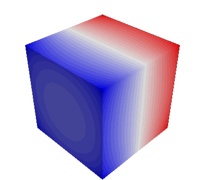
# Plot potential on the mesh
mlab.figure("Potential on the boundary", bgcolor=(1, 1, 1))
m = mlab.triangular_mesh(*mesh.vertices.T, mesh.faces, scalars=u, colormap="bwr")
m.actor.mapper.interpolate_scalars_before_mapping = True
m.module_manager.scalar_lut_manager.number_of_colors = 32
Out:
Computing input potential
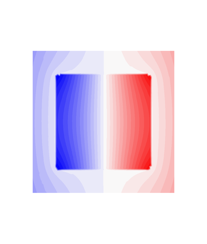
Load plane for the visualization of the potential
plane = load_example_mesh("10x10_plane_hires", process=True)
t = np.eye(4)
t[1:3, 1:3] = np.array([[0, 1], [-1, 0]])
plane.apply_transform(t)
plane.apply_scale(0.3)
plane = plane.subdivide()
Uplane = scalar_potential_coupling(
mesh, plane.vertices, multiply_coeff=False, approx_far=True
)
uprim = phi0x(plane.vertices)
usec = (mu_r - 1) / (4 * np.pi) * Uplane @ u
uplane = uprim + usec
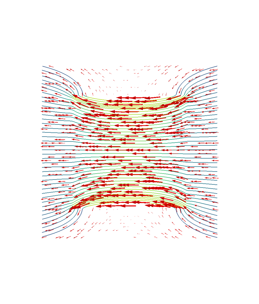
# Meshgrid on the same plane for the bfield
X, Y = np.meshgrid(
np.linspace(-1.5, 1.5, 50), np.linspace(-1.5, 1.5, 50), indexing="ij"
)
pp = np.zeros((50 * 50, 3))
pp[:, 0] = X.flatten()
pp[:, 1] = Y.flatten()
Bplane = magnetic_field_coupling(mesh, pp, analytic=True)
bprim = pp * 0 # copy pp
# add x directional field
mu0 = 1e-7 * 4 * np.pi
bprim[:, 0] = -1
# In this simulation mu0==1 is assumed
# magnetic_field_coupling uses mu0 in SI units
bplane = (mu_r - 1) / (4 * np.pi) / mu0 * Bplane @ u + bprim
# uplane[Uplane.sum(axis=1)]
Out:
Computing scalar potential coupling matrix, 2348 vertices by 6221 target points... took 4.16 seconds.
Computing magnetic field coupling matrix analytically, 2348 vertices by 2500 target points... took 7.62 seconds.
mlab.figure("Potential for B", bgcolor=(1, 1, 1), size=(1000, 1000))
m = mlab.triangular_mesh(*plane.vertices.T, plane.faces, scalars=uplane, colormap="bwr")
m.actor.mapper.interpolate_scalars_before_mapping = True
m.module_manager.scalar_lut_manager.number_of_colors = 32
# vectors = mlab.quiver3d(*(plane.triangles_center + np.array([0,0,0.001])).T,
#                         *(-gradient(uplane, plane)), color=(0,0,0),
#               scale_mode='none', scale_factor=0.01, mode='arrow')
# vectors.glyph.mask_input_points = True
# vectors.glyph.mask_points.random_mode_type = 0
# vectors.glyph.mask_points.on_ratio = 4
# vectors.glyph.glyph_source.glyph_position = 'center'
m.scene.z_plus_view()

mlab.figure("B field", bgcolor=(1, 1, 1), size=(1000, 1000))
vectors2 = mlab.quiver3d(
    *pp.T,
    *bplane.T,
    color=(1, 0, 0),
    scale_mode="vector",
    scale_factor=0.02,
    mode="arrow"
)
vectors2.glyph.glyph.scale_factor = 0.08
vectors2.glyph.mask_input_points = True
vectors2.glyph.mask_points.random_mode_type = 0
vectors2.glyph.mask_points.on_ratio = 4
vectors2.glyph.glyph_source.glyph_position = "center"
vectors2.scene.z_plus_view()

# Streamline plot for the cube
bplane[:, 2] = 0
vecfield = mlab.pipeline.vector_field(
    *pp.T.reshape(3, 50, 50, 1), *bplane.T.reshape(3, 50, 50, 1)
)
vecnorm = mlab.pipeline.extract_vector_norm(vecfield)
streams = []

Nq = 40
q = np.zeros((Nq, 3))
q[:, 1] = np.linspace(-1.5, 1.5, Nq)
q[:, 0] = 1.5
extent = np.array([-1.5, 1.5, -1.5, 1.5, 0, 0])
for qi in q:
    stream = mlab.pipeline.streamline(
        vecnorm,
        seed_scale=0.01,
        seedtype="point",
        integration_direction="both",
        extent=np.array([-1.5, 1.5, -1.5, 1.5, 0, 0]),
        colormap="viridis",
    )
    stream.stream_tracer.initial_integration_step = 0.1
    stream.stream_tracer.maximum_propagation = 200.0
    stream.seed.widget = stream.seed.widget_list[3]
    stream.seed.widget.position = qi
    stream.seed.widget.enabled = False  # hide the widget itself
    streams.append(stream)
Total running time of the script: ( 0 minutes 32.044 seconds)
Estimated memory usage: 2613 MB