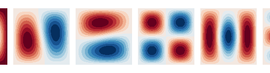
Visualize SUH components on 3 surfaces

import numpy as np
import matplotlib.pyplot as plt
from mayavi import mlab
import trimesh

from bfieldtools.suhtools import SuhBasis
from bfieldtools.utils import find_mesh_boundaries

from trimesh.creation import icosphere
from bfieldtools.utils import load_example_mesh

# Import meshes

# Sphere
sphere = icosphere(4, 0.1)

# Plane mesh centered on the origin
plane = load_example_mesh("10x10_plane_hires")
scaling_factor = 0.02
plane.apply_scale(scaling_factor)
# Rotate to x-plane
t = np.eye(4)
t[1:3, 1:3] = np.array([[0, 1], [-1, 0]])
plane.apply_transform(t)

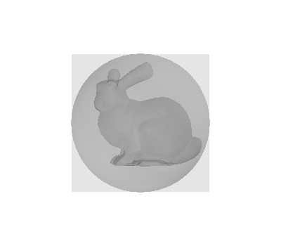
# Bunny
bunny = load_example_mesh("bunny_repaired")
bunny.vertices -= bunny.vertices.mean(axis=0)

mlab.figure(bgcolor=(1, 1, 1))
for mesh in (sphere, plane, bunny):
    s = mlab.triangular_mesh(
        *mesh.vertices.T, mesh.faces, color=(0.5, 0.5, 0.5), opacity=0.2
    )
s.scene.z_plus_view()

Nc = 20
basis_sphere = SuhBasis(sphere, Nc)
basis_plane = SuhBasis(plane, Nc)
basis_bunny = SuhBasis(bunny, Nc)


A = [mesh.area for mesh in (bunny, sphere, plane)]

Out:

Calculating surface harmonics expansion...
Computing the laplacian matrix...
Computing the mass matrix...
Closed mesh or Neumann BC, leaving out the constant component
Calculating surface harmonics expansion...
Computing the laplacian matrix...
Computing the mass matrix...
Calculating surface harmonics expansion...
Computing the laplacian matrix...
Computing the mass matrix...
Closed mesh or Neumann BC, leaving out the constant component

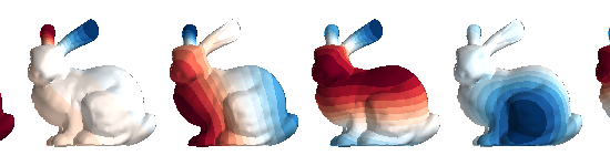
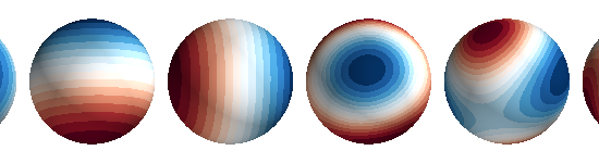
Nfuncs = [0, 1, 2, 3, 4, 5]
kwargs = {"colormap": "RdBu", "ncolors": 15}
plt.figure(figsize=(3.5, 2.5))
for i, b in enumerate((basis_bunny, basis_sphere, basis_plane)):
    fig = mlab.figure(bgcolor=(1, 1, 1), size=(550, 150))
    s = b.plot(Nfuncs, 0.1, Ncols=6, figure=fig, **kwargs)
    s[0].scene.parallel_projection = True
    s[0].scene.z_plus_view()
    if i == 0:
        s[0].scene.camera.parallel_scale = 0.1
    else:
        s[0].scene.camera.parallel_scale = 0.13
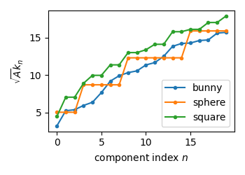
    plt.plot(np.sqrt(b.eigenvals * A[i]), ".-")

plt.legend(("bunny", "sphere", "square"), loc="lower right")
plt.xlabel("component index $n$")
plt.ylabel("$\sqrt{A}k_n$")
plt.tight_layout()

• 
• 
• 

Out:

0 0
1 0
2 0
3 0
4 0
5 0
0 0
1 0
2 0
3 0
4 0
5 0
0 0
1 0
2 0
3 0
4 0
5 0

Estimated memory usage: 12 MB