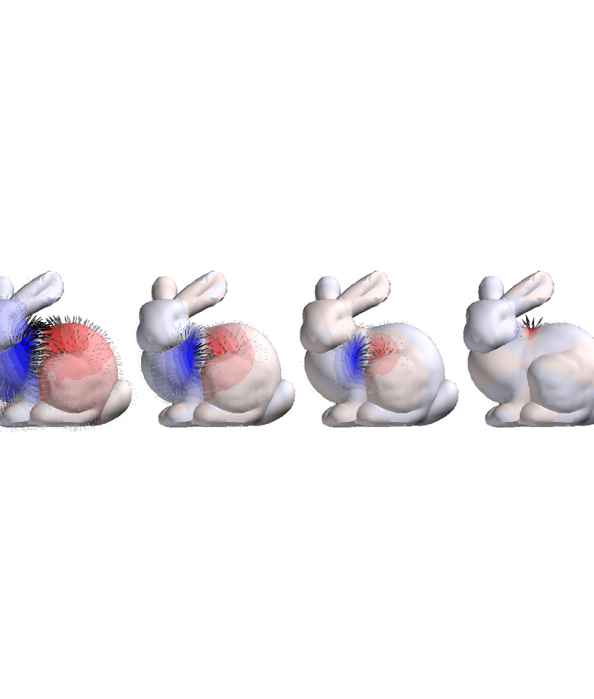
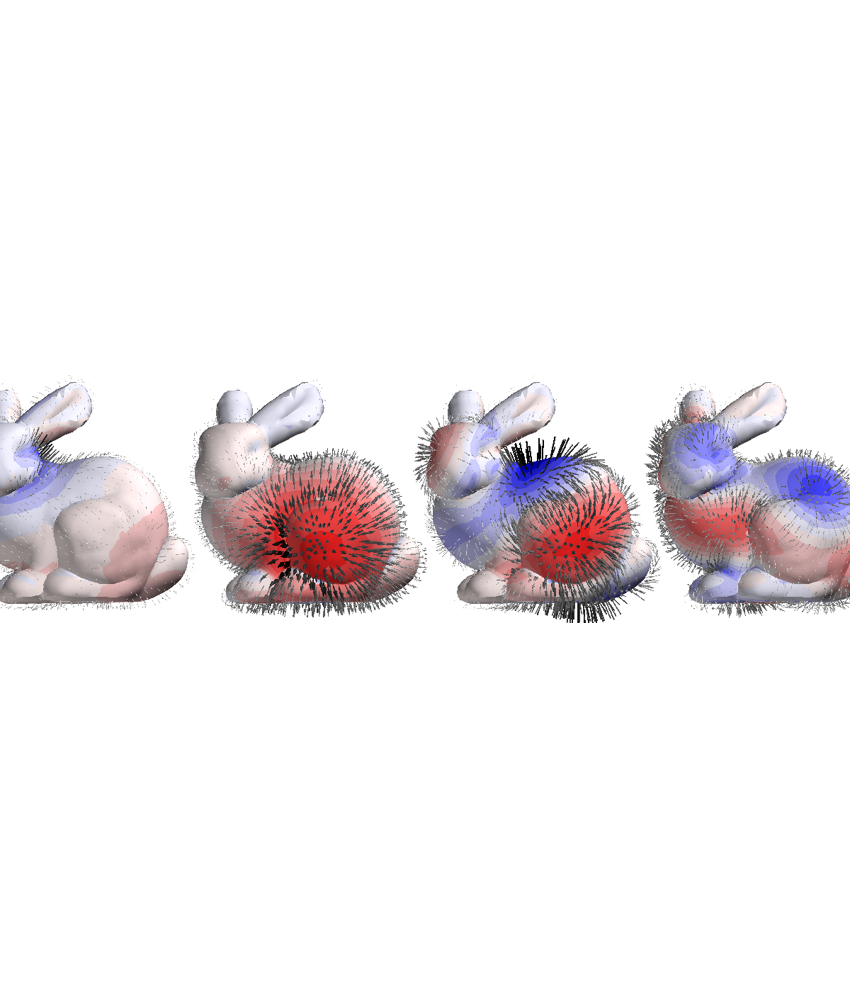
Compare SUH and SPH basis functions for the magnetic field

import numpy as np
import matplotlib.pyplot as plt
from mayavi import mlab
import trimesh
import pkg_resources
from pyface.api import GUI

_gui = GUI()


from bfieldtools.mesh_magnetics import magnetic_field_coupling
from bfieldtools.mesh_magnetics import magnetic_field_coupling_analytic
from bfieldtools.mesh_magnetics import scalar_potential_coupling
from bfieldtools.sphtools import compute_sphcoeffs_mesh, basis_fields
from bfieldtools.suhtools import SuhBasis
from bfieldtools.utils import load_example_mesh


mesh = load_example_mesh("bunny_repaired")

mesh.vertices -= mesh.vertices.mean(axis=0)

mesh_field = mesh.copy()
mesh_field.vertices += 0.005 * mesh_field.vertex_normals
mesh_field = trimesh.smoothing.filter_laplacian(mesh_field, iterations=1)

Ca, Cb = basis_fields(mesh_field.vertices, 4)

bsuh = SuhBasis(mesh, 25)
Csuh = magnetic_field_coupling_analytic(mesh, mesh_field.vertices) @ bsuh.basis

Out:

Calculating surface harmonics expansion...
Computing the laplacian matrix...
Computing the mass matrix...
Closed mesh or Neumann BC, leaving out the constant component
Computing magnetic field coupling matrix analytically, 2503 vertices by 2503 target points... took 8.26 seconds.

def plot_basis_fields(C, comps):
    d = 0.17
    i = 0
    j = 0
    for n in comps:
        p = 1.05 * mesh_field.vertices.copy()
        p2 = mesh_field.vertices.copy()
        #        p[:,1] -= i*d
        #        p2[:,1] -= i*d
        p[:, 0] += i * d
        p2[:, 0] += i * d
        m = np.max(np.linalg.norm(C[:, :, n], axis=0))
        vectors = mlab.quiver3d(
            *p.T, *C[:, :, n].T, mode="arrow", colormap="Greys", vmin=0, vmax=m
        )
        vectors.glyph.mask_input_points = True
        vectors.glyph.mask_points.maximum_number_of_points = 1800
        vectors.glyph.mask_points.random_mode_type = 1
        vectors.glyph.glyph_source.glyph_position = "center"
        vectors.glyph.glyph_source.glyph_source.shaft_radius = 0.02
        vectors.glyph.glyph_source.glyph_source.tip_radius = 0.06
        vectors.glyph.glyph.scale_factor = 0.03
        #        m = np.max(abs((C[:,:,n].T*mesh_field.vertex_normals.T).sum(axis=0)))
        #        s =mlab.triangular_mesh(*p.T, mesh_field.faces,
        #                             scalars=(C[:,:,n].T*mesh_field.vertex_normals.T).sum(axis=0),
        #                             colormap='seismic', vmin=-m, vmax=m, opacity=0.7)
        #        s.actor.property.backface_culling = True
        m = np.max(abs((C[:, :, n].T * mesh_field.vertex_normals.T).sum(axis=0)))
        s = mlab.triangular_mesh(
            *p2.T,
            mesh.faces,
            scalars=(C[:, :, n].T * mesh_field.vertex_normals.T).sum(axis=0),
            colormap="bwr",
            vmin=-m,
            vmax=m
        )
        s.actor.mapper.interpolate_scalars_before_mapping = True
        s.module_manager.scalar_lut_manager.number_of_colors = 15
        i += 1


comps = [0, 4, 10, 15]
scene = mlab.figure(bgcolor=(1, 1, 1), size=(1200, 350))
plot_basis_fields(Ca, comps)
scene.scene.parallel_projection = True
scene.scene.z_plus_view()
scene.scene.camera.zoom(4)
while scene.scene.light_manager is None:
    _gui.process_events()
scene.scene.light_manager.lights[2].intensity = 0.2


scene = mlab.figure(bgcolor=(1, 1, 1), size=(1200, 350))
plot_basis_fields(Csuh, comps)
scene.scene.parallel_projection = True
scene.scene.z_plus_view()
scene.scene.camera.zoom(4)
while scene.scene.light_manager is None:
    _gui.process_events()
scene.scene.light_manager.lights[2].intensity = 0.2

• 
• 

from bfieldtools.mesh_magnetics import scalar_potential_coupling

scaling_factor = 0.02

#Load simple plane mesh that is centered on the origin

file_obj=pkg_resources.resource_filename(‘bfieldtools’, ‘example_meshes/10x10_plane_hires.obj’) plane = trimesh.load(file_obj=file_obj, process=False) plane.apply_scale(scaling_factor)

# Rotate to x-plane

t = np.eye(4) t[1:3,1:3] = np.array([[0,1],[-1,0]]) plane.apply_transform(t) plane = plane.subdivide()

u = scalar_potential_coupling(mesh, plane.vertices, multiply_coeff=False) mask = 1 + np.sum(u, axis=1)/(4*np.pi) mask[mask < 1e-6] = 0

Ca, Cb = basis_fields(plane.vertices, 6) bsuh = SuhBasis(mesh, 48) CB = magnetic_field_coupling_analytic(mesh, plane.vertices) Csuh = CB @ bsuh.basis

A,B = compute_sphcoeffs_mesh(mesh, 6) b1 = np.einsum(‘ij,lik->lkj’, A , Ca) # Mapping from verts to alpha to field b2 = np.einsum(‘ij,klj->lki’, bsuh.mass @ bsuh.basis , Csuh) # Mapping from verts to suh to field

ind=1932 scalars = np.zeros(mesh.vertices.shape[0]) scalars[ind] = 1 mlab.triangular_mesh(*mesh.vertices.T, mesh.faces, scalars=scalars, colormap=’Blues’) surf= mlab.triangular_mesh(*plane.vertices.T, plane.faces, colormap=’viridis’,

scalars = mask*np.linalg.norm(CB[:,:,ind], axis=1))

surf.actor.mapper.interpolate_scalars_before_mapping = True surf.module_manager.scalar_lut_manager.number_of_colors = 16

mlab.figure() mlab.triangular_mesh(*mesh.vertices.T, mesh.faces, scalars=scalars, colormap=’Blues’) surf = mlab.triangular_mesh(*plane.vertices.T, plane.faces, colormap=’viridis’,

scalars = mask*np.linalg.norm(b1[:,:,ind], axis=0))

surf.actor.mapper.interpolate_scalars_before_mapping = True surf.module_manager.scalar_lut_manager.number_of_colors = 16

mlab.figure() mlab.triangular_mesh(*mesh.vertices.T, mesh.faces, scalars=scalars, colormap=’Blues’) surf = mlab.triangular_mesh(*plane.vertices.T, plane.faces, colormap=’viridis’,

scalars = mask*np.linalg.norm(b2[:,:,ind], axis=0))

surf.actor.mapper.interpolate_scalars_before_mapping = True surf.module_manager.scalar_lut_manager.number_of_colors = 16

Estimated memory usage: 792 MB