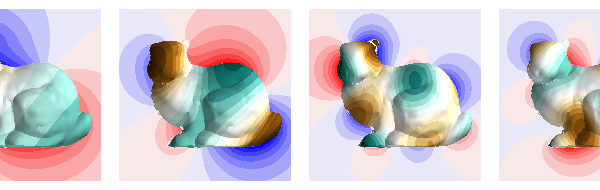
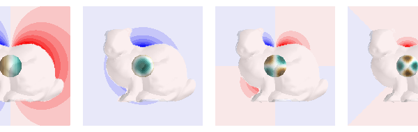
Compare SUH and SPH basis functions for the magnetic scalar potential

import numpy as np
import matplotlib.pyplot as plt
from mayavi import mlab
import trimesh
import pkg_resources
from pyface.api import GUI

_gui = GUI()


from bfieldtools.mesh_magnetics import magnetic_field_coupling
from bfieldtools.mesh_magnetics import magnetic_field_coupling_analytic
from bfieldtools.mesh_magnetics import scalar_potential_coupling
from bfieldtools.sphtools import compute_sphcoeffs_mesh, basis_fields
from bfieldtools.suhtools import SuhBasis
from bfieldtools.utils import load_example_mesh


mesh = load_example_mesh("bunny_repaired", process=True)

mesh.vertices -= mesh.vertices.mean(axis=0)

mesh_field = mesh.copy()
mesh_field.vertices += 0.001 * mesh_field.vertex_normals
# mesh_field = trimesh.smoothing.filter_laplacian(mesh_field, iterations=1)

# Ca, Cb = basis_fields(mesh_field.vertices, 4)

# bsuh = SuhBasis(mesh, 25)
# Csuh = magnetic_field_coupling_analytic(mesh, mesh_field.vertices) @ bsuh.basis

def plot_basis_fields(C, comps):

d = 0.17 i = 0 j = 0 for n in comps:

p = 1.05 * mesh_field.vertices.copy() p2 = mesh_field.vertices.copy() # p[:,1] -= i*d # p2[:,1] -= i*d p[:, 0] += i * d p2[:, 0] += i * d m = np.max(np.linalg.norm(C[:, :, n], axis=0)) vectors = mlab.quiver3d(

*p.T, *C[:, :, n].T, mode=”arrow”, colormap=”Greys”, vmin=0, vmax=m

) vectors.glyph.mask_input_points = True vectors.glyph.mask_points.maximum_number_of_points = 1800 vectors.glyph.mask_points.random_mode_type = 1 vectors.glyph.glyph_source.glyph_position = “center” vectors.glyph.glyph_source.glyph_source.shaft_radius = 0.02 vectors.glyph.glyph_source.glyph_source.tip_radius = 0.06 vectors.glyph.glyph.scale_factor = 0.03 # m = np.max(abs((C[:,:,n].T*mesh_field.vertex_normals.T).sum(axis=0))) # s =mlab.triangular_mesh(*p.T, mesh_field.faces, # scalars=(C[:,:,n].T*mesh_field.vertex_normals.T).sum(axis=0), # colormap=’seismic’, vmin=-m, vmax=m, opacity=0.7) # s.actor.property.backface_culling = True m = np.max(abs((C[:, :, n].T * mesh_field.vertex_normals.T).sum(axis=0))) s = mlab.triangular_mesh(

*p2.T, mesh.faces, scalars=(C[:, :, n].T * mesh_field.vertex_normals.T).sum(axis=0), colormap=”bwr”, vmin=-m, vmax=m

) s.actor.mapper.interpolate_scalars_before_mapping = True s.module_manager.scalar_lut_manager.number_of_colors = 15 i += 1

# comps = [0, 4, 10, 15]
# scene = mlab.figure(bgcolor=(1, 1, 1), size=(1200, 350))
# plot_basis_fields(Ca, comps)
# scene.scene.parallel_projection = True
# scene.scene.z_plus_view()
# scene.scene.camera.zoom(4)
# while scene.scene.light_manager is None:
#     _gui.process_events()
# scene.scene.light_manager.lights[2].intensity = 0.2


# scene = mlab.figure(bgcolor=(1, 1, 1), size=(1200, 350))
# plot_basis_fields(Csuh, comps)
# scene.scene.parallel_projection = True
# scene.scene.z_plus_view()
# scene.scene.camera.zoom(4)
# while scene.scene.light_manager is None:
#     _gui.process_events()
# scene.scene.light_manager.lights[2].intensity = 0.2

from bfieldtools.mesh_magnetics import scalar_potential_coupling
from bfieldtools.sphtools import basis_potentials

scaling_factor = 0.02
# Load simple plane mesh that is centered on the origin
plane = load_example_mesh("10x10_plane_hires")
plane.apply_scale(scaling_factor)
# Rotate to x-plane
t = np.eye(4)
t[1:3, 1:3] = np.array([[0, 1], [-1, 0]])
plane.apply_transform(t)
# Subdivide face close to the mesh
from trimesh.proximity import signed_distance

dd = signed_distance(mesh, plane.triangles_center)
plane = plane.subdivide(np.flatnonzero(abs(dd) < 0.005))
dd = signed_distance(mesh, plane.triangles_center)
plane = plane.subdivide(np.flatnonzero(abs(dd) < 0.002))

UB = scalar_potential_coupling(mesh, plane.vertices, multiply_coeff=False)
mask = np.sum(UB, axis=1)
mask = mask > -0.5

Ua, Ub = basis_potentials(plane.vertices, 6)
bsuh = SuhBasis(mesh, 48)
# UB = scalar_potential_coupling(mesh, plane.vertices)
Usuh = UB @ bsuh.basis

sphere = trimesh.creation.icosphere(radius=0.02)
Ua_mesh, Ub_mesh = basis_potentials(sphere.vertices, 5)
UB_mesh = scalar_potential_coupling(mesh, mesh_field.vertices)
Usuh_mesh = UB_mesh @ bsuh.basis

Out:

Computing scalar potential coupling matrix, 2503 vertices by 3562 target points... took 11.10 seconds.
Calculating surface harmonics expansion...
Computing the laplacian matrix...
Computing the mass matrix...
Closed mesh or Neumann BC, leaving out the constant component
Computing scalar potential coupling matrix, 2503 vertices by 2503 target points... took 7.55 seconds.

comps = [0, 5, 13, 17]
d = 0.22
from bfieldtools.viz import plot_data_on_vertices
from bfieldtools.viz import plot_mesh

# Plot suh
i = 0
fig = mlab.figure(bgcolor=(1, 1, 1), size=(600, 190))
for n in comps:
    p = plane.copy()
    p.vertices[:, 0] += i * d
    p2 = mesh_field.copy()
    p2.vertices[:, 0] += i * d
    scalars = Usuh[:, n].copy()
    scalars[~mask] = 0
    scalars2 = bsuh.basis[:, n]
    m = np.max(abs(scalars))
    m2 = np.max(abs(scalars2))
    plot_data_on_vertices(p, scalars, figure=fig, ncolors=15, vmax=m, colormap="bwr")
    plot_data_on_vertices(
        p2, scalars2, figure=fig, ncolors=15, vmax=m2, colormap="BrBG"
    )
    i += 1
fig.scene.parallel_projection = True
fig.scene.z_plus_view()
fig.scene.camera.parallel_scale = 0.11

i = 0
fig = mlab.figure(bgcolor=(1, 1, 1), size=(600, 190))
for n in comps:
    p = plane.copy()
    p.vertices[:, 0] += i * d
    p2 = sphere.copy()
    p2.vertices[:, 0] += i * d
    scalars = Ua[:, n].copy()
    scalars[~mask] = 0
    scalars2 = Ua_mesh[:, n]
    m = np.max(abs(scalars))
    m2 = np.max(abs(scalars2))
    plot_data_on_vertices(p, scalars, figure=fig, ncolors=15, vmax=m, colormap="bwr")
    plot_data_on_vertices(
        p2, scalars2, figure=fig, ncolors=15, vmax=m2, colormap="BrBG"
    )
    p3 = mesh.copy()
    p3.vertices[:, 0] += i * d
    plot_mesh(p3, opacity=0.3, figure=fig)
    i += 1
fig.scene.parallel_projection = True
fig.scene.z_plus_view()
fig.scene.camera.parallel_scale = 0.11

Estimated memory usage: 652 MB