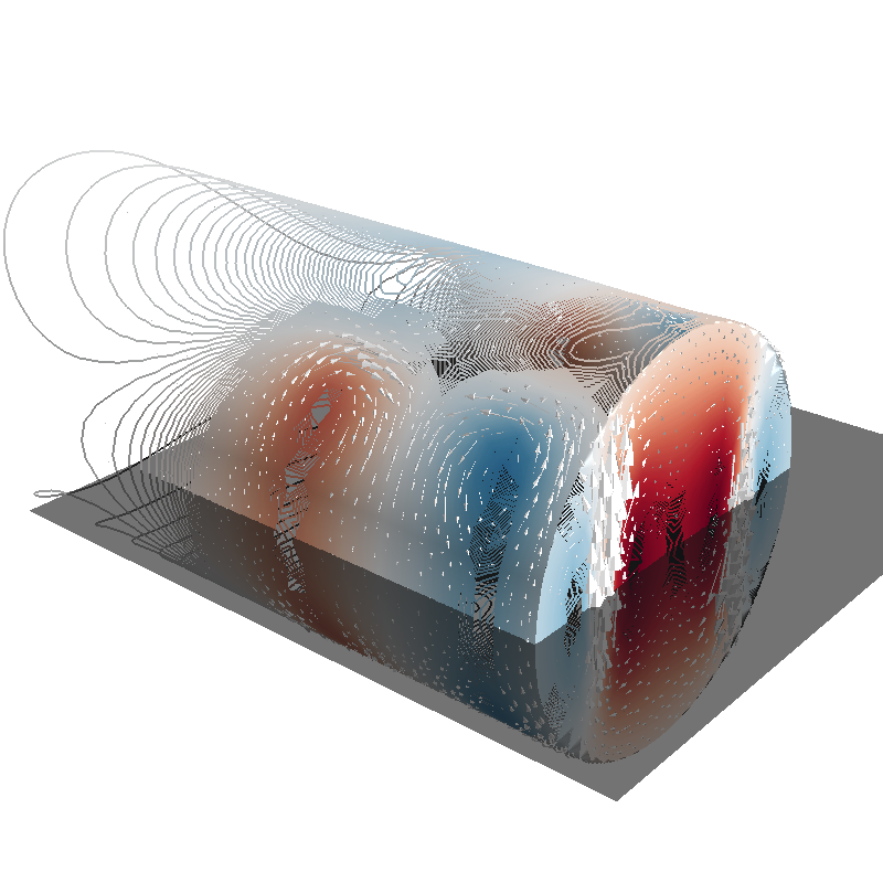
Field distortion by a perfect mu-metal shield

import numpy as np
import trimesh
from mayavi import mlab

from bfieldtools.mesh_conductor import MeshConductor, StreamFunction
from bfieldtools.mesh_calculus import gradient
from bfieldtools.utils import load_example_mesh, combine_meshes

# This doesn't matter, the problem is scale-invariant
scaling_factor = 1


planemesh = load_example_mesh("10x10_plane_hires")
planemesh.apply_scale(scaling_factor)

# Specify coil plane geometry
center_offset = np.array([9, 0, 0]) * scaling_factor
standoff = np.array([0, 4, 0]) * scaling_factor

# Create coil plane pairs
coil_plus = trimesh.Trimesh(
    planemesh.vertices + center_offset + standoff, planemesh.faces, process=False
)

coil_minus = trimesh.Trimesh(
    planemesh.vertices + center_offset - standoff, planemesh.faces, process=False
)

joined_planes = combine_meshes((coil_plus, coil_minus))
planemesh = joined_planes

# Create mesh class object
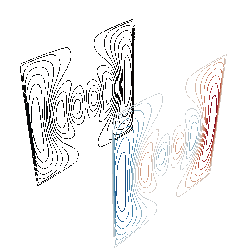
coil = MeshConductor(mesh_obj=joined_planes, fix_normals=True)

# Separate object for shield geometry
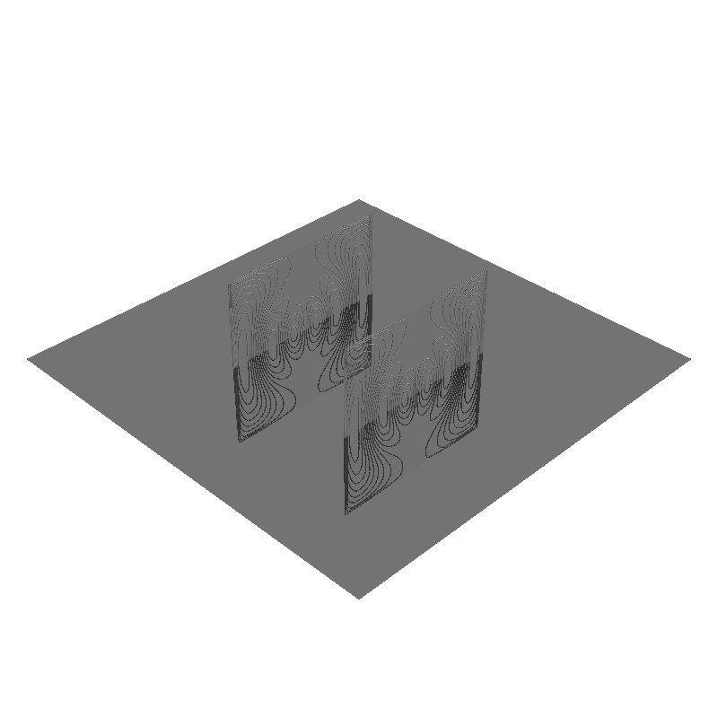
shieldmesh = load_example_mesh("closed_cylinder_remeshed")
shieldmesh.apply_scale(15)

shield = MeshConductor(mesh_obj=shieldmesh, process=True, fix_normals=True)

N = 80
points = np.zeros((N * N, 3))
w = 12
X, Y = np.meshgrid(np.linspace(-w, w, N), np.linspace(-w, w, N), indexing="ij")
X += planemesh.vertices.mean(axis=0)[0]
Y += planemesh.vertices.mean(axis=0)[1]
points[:, 0] = X.flatten()
points[:, 1] = Y.flatten()
points[:, 2] += planemesh.vertices.mean(axis=0)[2]


def plot_plane():
    mlab.triangular_mesh(
        [X.min(), X.max(), X.max(), X.min()],
        [Y.min(), Y.min(), Y.max(), Y.max()],
        np.zeros(4),
        np.array([[0, 1, 2], [2, 3, 0]]),
        color=(0.1, 0.1, 0.1),
        opacity=0.6,
    )

fig = mlab.figure(bgcolor=(1, 1, 1))
s0 = mlab.triangular_mesh(
    *shieldmesh.vertices.T, shieldmesh.faces, color=(0.5, 0.5, 0.5), opacity=0.3
)
s0.actor.property.backface_culling = False
s0.actor.property.ambient = 0.5

I_prim = np.load("../publication_software/Shielded coil/biplanar_streamfunction.npy")
sprim = StreamFunction(coil.vert2inner @ I_prim, coil)
m = max(abs(sprim))
s1 = sprim.plot(False, 16, vmin=-m, vmax=m)
s2 = sprim.plot(True, 20)
s2.actor.mapper.scalar_visibility = False
s2.actor.property.line_width = 1.2
# s2 = mlab.triangular_mesh(*planemesh.vertices.T, planemesh.faces, scalars=I_prim,
#                          colormap='RdBu')
# s2.enable_contours = True
# s2.contour.filled_contours = True
# s2.contour.number_of_contours = 20
s2.actor.property.render_lines_as_tubes = True
plot_plane()
scene = s0.module_manager
scene.scene.camera.position = [
    39.154871143623325,
    -40.509425675368334,
    26.56155776567048,
]
scene.scene.camera.focal_point = [
    4.239945673839333,
    1.041549923485209,
    -0.0005302515738243585,
]
scene.scene.camera.view_angle = 30.0
scene.scene.camera.view_up = [
    -0.28276020498745635,
    0.33658483701858727,
    0.898196701154387,
]
scene.scene.camera.clipping_range = [16.139073445910277, 116.31572537292347]
scene.scene.camera.compute_view_plane_normal()
scene.scene.render()

• 
• 
• 

%% Calculate primary potential matrix

Compute slightly inside

d = 1e-3
P_prim = coil.U_coupling(shieldmesh.vertices - d * shieldmesh.vertex_normals)

Out:

Computing scalar potential coupling matrix, 3184 vertices by 2773 target points... took 9.77 seconds.

mlab.figure()
s = mlab.triangular_mesh(
    *shieldmesh.vertices.T, shieldmesh.faces, scalars=P_prim @ sprim, opacity=1.0
)
s.enable_contours = True
s.contour.filled_contours = True
s.contour.number_of_contours = 30

%% Calculate linear collocation BEM matrix

P_shield = shield.U_coupling(shieldmesh.vertices - d * shieldmesh.vertex_normals)

Out:

Computing scalar potential coupling matrix, 2773 vertices by 2773 target points... took 8.82 seconds.

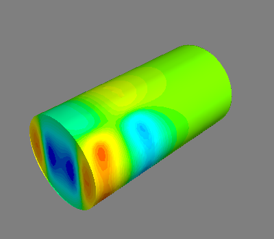
%% Solve equivalent stream function for the perfect linear mu-metal layer

I_shield = np.linalg.solve(-P_shield, P_prim @ sprim)
# I_shield = P_prim @ I_prim
s_shield = StreamFunction(I_shield, shield)
g = gradient(s_shield, shieldmesh, rotated=True)

fig = mlab.figure(bgcolor=(1, 1, 1))
s0 = mlab.triangular_mesh(
    *shieldmesh.vertices.T, shieldmesh.faces, color=(0.5, 0.5, 0.5), opacity=0.3
)
s0.actor.property.backface_culling = False
s1 = s_shield.plot(False, 256)
# s1.actor.property.opacity=0.8
s1.actor.property.backface_culling = False
# s2 = s_shield.plot(True, 10)
mlab.quiver3d(
    *shieldmesh.triangles_center.T,
    *g,
    color=(1, 1, 1),
    mode="arrow",
    scale_factor=0.0000008,
    scale_mode="vector"
)
# s1.contour.filled_contours = True
# s1.contour.number_of_contours = 30
# s2.actor.property.render_lines_as_tubes = True
# s1.actor.property.ambient = 0.2

scene = s1.module_manager
plot_plane()
scene.scene.camera.position = [
    39.154871143623325,
    -40.509425675368334,
    26.56155776567048,
]
scene.scene.camera.focal_point = [
    4.239945673839333,
    1.041549923485209,
    -0.0005302515738243585,
]
scene.scene.camera.view_angle = 30.0
scene.scene.camera.view_up = [
    -0.28276020498745635,
    0.33658483701858727,
    0.898196701154387,
]
scene.scene.camera.clipping_range = [16.139073445910277, 116.31572537292347]
scene.scene.camera.compute_view_plane_normal()
scene.scene.render()

• 
• 

U2_shield = shield.U_coupling(points)
U2_prim = coil.U_coupling(points)

Out:

Computing scalar potential coupling matrix, 2773 vertices by 6400 target points... took 20.79 seconds.
Computing scalar potential coupling matrix, 3184 vertices by 6400 target points... took 22.85 seconds.

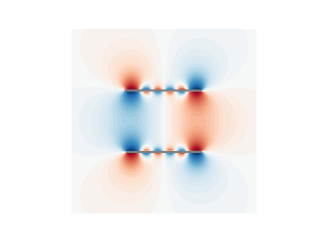
from bfieldtools.contour import scalar_contour

cc1 = scalar_contour(planemesh, planemesh.vertices[:, 2], contours=[-0.1])
cc1 = np.vstack(cc1)
cc1a = cc1[: cc1.shape[0] // 2]
cc1b = cc1[cc1.shape[0] // 2 :]
cc2 = scalar_contour(shieldmesh, shieldmesh.vertices[:, 2], contours=[-0.1])
cc2 = np.vstack(cc2)
cc2a = cc1[: cc2.shape[0] // 2]
cc2b = cc1[cc2.shape[0] // 2 :]

import matplotlib.pyplot as plt
import matplotlib.colors as colors


def truncate_colormap(cmap, minval=0.0, maxval=1.0, n=256):
    new_cmap = colors.LinearSegmentedColormap.from_list(
        "trunc({n},{a:.2f},{b:.2f})".format(n=cmap.name, a=minval, b=maxval),
        cmap(np.linspace(minval, maxval, n)),
    )
    return new_cmap


cmap = plt.get_cmap("RdBu")
# cmap.set_over((0.95,0.95,0.95))
# cmap.set_under((0.95,0.95,0.95))

u0 = abs(
    np.sum(U2_shield, axis=1).reshape(N, N)
)  # Solid angle of the shield, zero outside
u0 /= u0.max()
u0[u0 < 1e-6] = 0
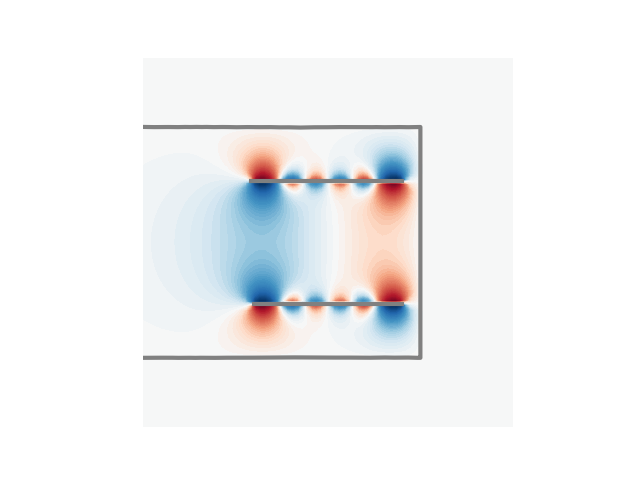
u1 = (U2_prim @ sprim).reshape(N, N)
u2 = (U2_shield @ I_shield).reshape(N, N) * u0
u3 = (u1 + u2) * u0

vmax = np.max(abs(u3)) * 0.99
levels = np.linspace(-vmax, vmax, 120)
levels = np.hstack((-np.max(abs(u3)), levels, np.max(abs(u3))))
p = plt.contourf(
    X,
    Y,
    u1,
    levels=levels,
    cmap=cmap,
    vmin=-vmax,
    vmax=vmax,
    norm=colors.SymLogNorm(linthresh=0.2 * vmax, linscale=0.8, vmin=-vmax, vmax=vmax),
)
plt.plot(cc1a[:, 0], cc1a[:, 1], linewidth=3, color="gray")
plt.plot(cc1b[:, 0], cc1b[:, 1], linewidth=3, color="gray")
plt.axis("image")
plt.axis("off")
xlims = p.ax.get_xlim()
plt.figure()
p = plt.contourf(
    X,
    Y,
    u2,
    levels=levels,
    cmap=cmap,
    vmin=-vmax,
    vmax=vmax,
    norm=colors.SymLogNorm(linthresh=0.2 * vmax, linscale=0.8, vmin=-vmax, vmax=vmax),
)
plt.plot(cc1a[:, 0], cc1a[:, 1], linewidth=3, color="gray")
plt.plot(cc1b[:, 0], cc1b[:, 1], linewidth=3, color="gray")
plt.plot(cc2[:, 0], cc2[:, 1], linewidth=3, color="gray")
plt.axis("image")
plt.axis("off")
p.ax.set_xlim(xlims)
plt.figure()
p = plt.contourf(
    X,
    Y,
    u3,
    levels=levels,
    cmap=cmap,
    vmin=-vmax,
    vmax=vmax,
    norm=colors.SymLogNorm(linthresh=0.2 * vmax, linscale=0.8, vmin=-vmax, vmax=vmax),
)
plt.plot(cc1a[:, 0], cc1a[:, 1], linewidth=3, color="gray")
plt.plot(cc1b[:, 0], cc1b[:, 1], linewidth=3, color="gray")
plt.plot(cc2[:, 0], cc2[:, 1], linewidth=3, color="gray")
plt.axis("image")
plt.axis("off")
p.ax.set_xlim(xlims)

• 
• 
• 

Out:

/home/rzetter/Documents/bfieldtools/examples/publication_physics/mumetal_shield_example.py:239: MatplotlibDeprecationWarning: default base may change from np.e to 10.  To suppress this warning specify the base keyword argument.
  norm=colors.SymLogNorm(linthresh=0.2 * vmax, linscale=0.8, vmin=-vmax, vmax=vmax),
/home/rzetter/Documents/bfieldtools/examples/publication_physics/mumetal_shield_example.py:255: MatplotlibDeprecationWarning: default base may change from np.e to 10.  To suppress this warning specify the base keyword argument.
  norm=colors.SymLogNorm(linthresh=0.2 * vmax, linscale=0.8, vmin=-vmax, vmax=vmax),
/home/rzetter/Documents/bfieldtools/examples/publication_physics/mumetal_shield_example.py:272: MatplotlibDeprecationWarning: default base may change from np.e to 10.  To suppress this warning specify the base keyword argument.
  norm=colors.SymLogNorm(linthresh=0.2 * vmax, linscale=0.8, vmin=-vmax, vmax=vmax),

(-2.9992466721105764, 21.000753327889424)

Estimated memory usage: 2103 MB