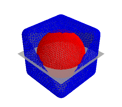
Design a field enclosed in a volume

import numpy as np
import matplotlib.pyplot as plt
from mayavi import mlab

# import trimesh

from bfieldtools.mesh_conductor import MeshConductor, StreamFunction
from bfieldtools.mesh_magnetics import magnetic_field_coupling as compute_C
from bfieldtools.mesh_magnetics import (
    magnetic_field_coupling_analytic as compute_C_analytic,
)
from bfieldtools.mesh_magnetics import scalar_potential_coupling as compute_U
from bfieldtools.mesh_impedance import mutual_inductance_matrix
from bfieldtools.contour import scalar_contour
from bfieldtools import sphtools
from bfieldtools.utils import load_example_mesh
from bfieldtools.mesh_calculus import mass_matrix

# domain = 'sphere'
# domain = 'cube'
domain = "combined"

if domain == "sphere":
    from trimesh.creation import icosphere

    mesh1 = icosphere(3, 0.65)
    mesh2 = icosphere(3, 0.8)
elif domain == "cube":
    from trimesh.creation import box
    from trimesh.smoothing import filter_laplacian

    mesh1 = box((1.0, 1.0, 1.0))
    mesh2 = box((1.5, 1.5, 1.5))

    for i in range(4):
        mesh1 = mesh1.subdivide()
        mesh2 = mesh2.subdivide()

    mesh1 = filter_laplacian(mesh1)
    mesh2 = filter_laplacian(mesh2, 0.9)
elif domain == "combined":
    from trimesh.creation import icosphere

    mesh1 = icosphere(4, 0.65)
    mesh2 = load_example_mesh("cube_fillet")
    mesh2.vertices -= mesh2.vertices.mean(axis=0)
    mesh2.vertices *= 0.15
#    mesh2 = mesh2.subdivide()

coil1 = MeshConductor(
    mesh_obj=mesh1,
    N_sph=3,
    inductance_nchunks=100,
    fix_normals=False,
    inductance_quad_degree=2,
)
coil2 = MeshConductor(
    mesh_obj=mesh2,
    N_sph=3,
    inductance_nchunks=100,
    fix_normals=False,
    inductance_quad_degree=2,
)

M11 = coil1.inductance
M22 = coil2.inductance
# Add rank-one matrix, so that M22 can be inverted
M22 += np.ones_like(M22) / M22.shape[0] * np.mean(np.diag(M22))
M11 += np.ones_like(M11) / M11.shape[0] * np.mean(np.diag(M11))
M21 = mutual_inductance_matrix(mesh2, mesh1)

M = np.block([[M11, M21.T], [M21, M22]])


x = y = np.linspace(-0.85, 0.85, 100)
X, Y = np.meshgrid(x, y, indexing="ij")
points = np.zeros((X.flatten().shape[0], 3))
points[:, 0] = X.flatten()
points[:, 1] = Y.flatten()

CB1 = compute_C_analytic(mesh1, points)
CB2 = compute_C_analytic(mesh2, points)

CU1 = compute_U(mesh1, points)
CU2 = compute_U(mesh2, points)

Out:

Computing the inductance matrix...
Computing self-inductance matrix using rough quadrature (degree=2).              For higher accuracy, set quad_degree to 4 or more.
Computing triangle-coupling matrix
Inductance matrix computation took 15.33 seconds.
Computing the inductance matrix...
Computing self-inductance matrix using rough quadrature (degree=2).              For higher accuracy, set quad_degree to 4 or more.
Computing triangle-coupling matrix
Inductance matrix computation took 11.63 seconds.
Estimating 24888 MiB required for 2665 by 2562 vertices...
Computing inductance matrix in 340 chunks (1485 MiB memory free),              when approx_far=True using more chunks is faster...
Computing triangle-coupling matrix
Computing magnetic field coupling matrix analytically, 2562 vertices by 10000 target points... took 43.93 seconds.
Computing magnetic field coupling matrix analytically, 2665 vertices by 10000 target points... took 38.57 seconds.
Computing scalar potential coupling matrix, 2562 vertices by 10000 target points... took 30.87 seconds.
Computing scalar potential coupling matrix, 2665 vertices by 10000 target points... took 31.94 seconds.

suh = SuhBasis(mesh1, 100)

b10 = mesh1.vertex_normals[:, 0] b20 = (

mesh1.vertex_normals[:, 0] * mesh1.vertices[:, 0] - mesh1.vertex_normals[:, 1] * mesh1.vertices[:, 1]

)

N = mass_matrix(mesh1, lumped=True)
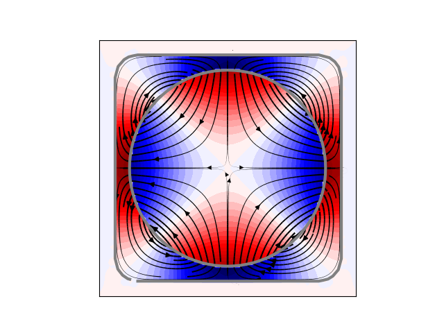
af, bf = sphtools.basis_fields(mesh1.vertices, 2)
b1 = N @ np.sum(bf[:, :, 2] * mesh1.vertex_normals, axis=1)
b2 = N @ np.sum(bf[:, :, 3] * mesh1.vertex_normals, axis=1)


def plot_plane(opacity=0.8):
    mlab.triangular_mesh(
        np.array([x[0], x[-1], x[-1], x[0]]),
        np.array([x[0], x[0], x[-1], x[-1]]),
        np.zeros(4),
        np.array([[0, 1, 2], [2, 3, 0]]),
        color=(0.7, 0.7, 0.7),
        opacity=opacity,
    )


for bi in (b1, b2):

    bb = np.zeros(M.shape[1])
    bb[: M11.shape[1]] = bi
    I = np.linalg.solve(M, bb)
    I1 = I[: M11.shape[1]]
    I2 = I[M11.shape[1] :]

    B1 = CB1 @ I1
    B2 = CB2 @ I2

    U1 = CU1 @ I1
    U2 = CU2 @ I2

    # Plot
    # Extract the cross-sections of the plane and the surfaces
    cc1 = scalar_contour(mesh1, mesh1.vertices[:, 2], contours=[-0.001])[0]
    cc2 = scalar_contour(mesh2, mesh2.vertices[:, 2], contours=[-0.001])[0]

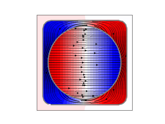
    B = (B1.T + B2.T)[:2].reshape(2, x.shape[0], y.shape[0])
    lw = np.sqrt(B[0] ** 2 + B[1] ** 2)
    lw = 2 * lw / np.max(lw)
    xx = np.linspace(-1, 1, 16)
    # seed_points = 0.51*np.array([xx, -np.sqrt(1-xx**2)])
    # seed_points = np.hstack([seed_points, (0.51*np.array([xx, np.sqrt(1-xx**2)]))])
    seed_points = np.array([cc1[:, 0], cc1[:, 1]]) * 1.01
    # plt.streamplot(x,y, B[1], B[0], density=2, linewidth=lw, color='k',
    #               start_points=seed_points.T, integration_direction='both')
    U = (U1 + U2).reshape(x.shape[0], y.shape[0])
    U /= np.max(U)
    plt.figure()
    plt.contourf(X, Y, U.T, cmap="seismic", levels=40)
    # plt.imshow(U, vmin=-1.0, vmax=1.0, cmap='seismic', interpolation='bicubic',
    #           extent=(x.min(), x.max(), y.min(), y.max()))
    plt.streamplot(
        x,
        y,
        B[1],
        B[0],
        density=2,
        linewidth=lw,
        color="k",
        start_points=seed_points.T,
        integration_direction="both",
    )

    plt.plot(cc1[:, 1], cc1[:, 0], linewidth=3.0, color="gray")
    plt.plot(cc2[:, 1], cc2[:, 0], linewidth=3.0, color="gray")

    plt.xticks([])
    plt.yticks([])

    plt.axis("image")

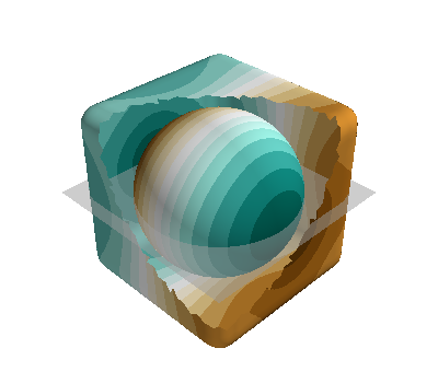
    # Plot "coils"
    mlab.figure(bgcolor=(1, 1, 1))
    contours1 = scalar_contour(mesh1, I1, 12)
    contours2 = scalar_contour(mesh2, I2, 12)

    #    fig = plot_3d_current_loops(contours1, tube_radius=0.005, colors=(1,1,1))
    surf = mlab.triangular_mesh(
        *mesh1.vertices.T, mesh1.faces, scalars=I1, colormap="BrBG"
    )
    surf.actor.mapper.interpolate_scalars_before_mapping = True
    surf.module_manager.scalar_lut_manager.number_of_colors = 16

    #    plot_3d_current_loops(contours2, tube_radius=0.005, figure=fig, colors=(0,0,0))
    faces2_masked = mesh2.faces[
        np.linalg.norm(mesh2.triangles_center - np.array([0.75, 0.75, 0.75]), axis=1)
        > 1.2
    ]
    surf = mlab.triangular_mesh(
        *(mesh2.vertices * 0.99).T,
        faces2_masked,
        scalars=I2,
        colormap="BrBG",
        opacity=1.0
    )
    surf.actor.mapper.interpolate_scalars_before_mapping = True
    surf.module_manager.scalar_lut_manager.number_of_colors = 16
    plot_plane(0.5)

• 
• 

• 
• 

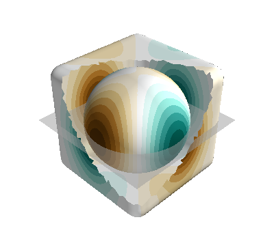
mlab.figure(bgcolor=(1, 1, 1))
s1 = mlab.triangular_mesh(
    *mesh1.vertices.T, mesh1.faces[:, ::-1], color=(0.5, 0.5, 0.5), opacity=1.0
)
s1.actor.property.backface_culling = True
w1 = mlab.triangular_mesh(
    *(mesh1.vertices.T + 0.009 * mesh1.vertex_normals.T),
    mesh1.faces,
    color=(1, 0, 0,),
    representation="wireframe"
)
w1.actor.property.render_lines_as_tubes = True

s2 = mlab.triangular_mesh(
    *mesh2.vertices.T, mesh2.faces[:, ::-1], color=(0.5, 0.5, 0.5), opacity=1.0
)
s2.actor.property.backface_culling = True
faces2_masked = mesh2.faces[(mesh2.triangles_center @ np.array([1, 1, 1])) < 1]
w2 = mlab.triangular_mesh(
    *(mesh2.vertices.T + +0.009 * mesh2.vertex_normals.T),
    faces2_masked,
    representation="wireframe",
    color=(0, 0, 1)
)
w2.actor.property.render_lines_as_tubes = True
plot_plane()

Estimated memory usage: 4267 MB