Example of designing a shielded biplanar coil

import numpy as np
import matplotlib.pyplot as plt
from mayavi import mlab
import trimesh

from bfieldtools.mesh_conductor import MeshConductor, StreamFunction
from bfieldtools.contour import scalar_contour
from bfieldtools.viz import plot_3d_current_loops
from bfieldtools.utils import load_example_mesh, combine_meshes


# Set unit, e.g. meter or millimeter.
# This doesn't matter, the problem is scale-invariant
scaling_factor = 0.1

# Load simple plane mesh that is centered on the origin
planemesh = load_example_mesh("10x10_plane_hires")
planemesh.apply_scale(scaling_factor)

# Specify coil plane geometry
center_offset = np.array([0, 0, 0]) * scaling_factor
standoff = np.array([0, 4, 0]) * scaling_factor

# Create coil plane pairs
coil_plus = trimesh.Trimesh(
    planemesh.vertices + center_offset + standoff, planemesh.faces, process=False
)

coil_minus = trimesh.Trimesh(
    planemesh.vertices + center_offset - standoff, planemesh.faces, process=False
)

mesh1 = combine_meshes((coil_minus, coil_plus))
mesh2 = mesh1.copy()
mesh2.apply_scale(1.4)

coil1 = MeshConductor(mesh_obj=mesh1, basis_name="inner", N_sph=4)
coil2 = MeshConductor(mesh_obj=mesh2, basis_name="inner", N_sph=4)

M11 = coil1.inductance
M22 = coil2.inductance
M21 = coil2.mutual_inductance(coil1)
# Mapping from I1 to I2, constraining flux through mesh2 to zero
P = -np.linalg.solve(M22, M21)

A1, Beta1 = coil1.sph_couplings
A2, Beta2 = coil2.sph_couplings

# Use lines below to get coulings with different normalization
# from bfieldtools.sphtools import compute_sphcoeffs_mesh
# A1, Beta1 = compute_sphcoeffs_mesh(mesh1, 5, normalization='energy', R=1)
# A2, Beta2 = compute_sphcoeffs_mesh(mesh2, 5, normalization='energy', R=1)

# Beta1 = Beta1[:, coil1.inner_vertices]
# Beta2 = Beta2[:, coil2.inner_vertices]

x = y = np.linspace(-0.8, 0.8, 50)  # 150)
X, Y = np.meshgrid(x, y, indexing="ij")
points = np.zeros((X.flatten().shape[0], 3))
points[:, 0] = X.flatten()
points[:, 1] = Y.flatten()


CB1 = coil1.B_coupling(points)
CB2 = coil2.B_coupling(points)

CU1 = coil1.U_coupling(points)
CU2 = coil2.U_coupling(points)

Out:

Computing the inductance matrix...
Computing self-inductance matrix using rough quadrature (degree=2).              For higher accuracy, set quad_degree to 4 or more.
Estimating 34964 MiB required for 3184 by 3184 vertices...
Computing inductance matrix in 60 chunks (12500 MiB memory free),              when approx_far=True using more chunks is faster...
Computing triangle-coupling matrix
Inductance matrix computation took 12.91 seconds.
Computing the inductance matrix...
Computing self-inductance matrix using rough quadrature (degree=2).              For higher accuracy, set quad_degree to 4 or more.
Estimating 34964 MiB required for 3184 by 3184 vertices...
Computing inductance matrix in 60 chunks (12289 MiB memory free),              when approx_far=True using more chunks is faster...
Computing triangle-coupling matrix
Inductance matrix computation took 13.15 seconds.
Estimating 34964 MiB required for 3184 by 3184 vertices...
Computing inductance matrix in 60 chunks (12118 MiB memory free),              when approx_far=True using more chunks is faster...
Computing triangle-coupling matrix
Computing coupling matrices
l = 1 computed
l = 2 computed
l = 3 computed
l = 4 computed
Computing coupling matrices
l = 1 computed
l = 2 computed
l = 3 computed
l = 4 computed
Computing magnetic field coupling matrix, 3184 vertices by 2500 target points... took 1.80 seconds.
Computing magnetic field coupling matrix, 3184 vertices by 2500 target points... took 1.80 seconds.
Computing scalar potential coupling matrix, 3184 vertices by 2500 target points... took 8.65 seconds.
Computing scalar potential coupling matrix, 3184 vertices by 2500 target points... took 8.68 seconds.

alpha[15] = 1 Minimization of magnetic energy with spherical harmonic constraint

C = Beta1 + Beta2 @ P
M = M11 + M21.T @ P

from scipy.linalg import eigvalsh

ssmax = eigvalsh(C.T @ C, M, eigvals=[M.shape[1] - 1, M.shape[1] - 1])

beta = np.zeros(Beta1.shape[0])
beta[7] = 1  # Gradient
# beta[2] = 1  # Homogeneous

# Minimum residual
_lambda = 1e3
# Minimum energy
# _lambda=1e-3
I1inner = np.linalg.solve(C.T @ C + M * ssmax / _lambda, C.T @ beta)

I2inner = P @ I1inner

s1 = StreamFunction(I1inner, coil1)
s2 = StreamFunction(I2inner, coil2)

# s = mlab.triangular_mesh(*mesh1.vertices.T, mesh1.faces, scalars=I1)
# s.enable_contours=True
# s = mlab.triangular_mesh(*mesh2.vertices.T, mesh2.faces, scalars=I2)
# s.enable_contours=True

B1 = CB1 @ s1
B2 = CB2 @ s2

U1 = CU1 @ s1
U2 = CU2 @ s2

cc1 = scalar_contour(mesh1, mesh1.vertices[:, 2], contours=[-0.001])
cc2 = scalar_contour(mesh2, mesh2.vertices[:, 2], contours=[-0.001])
cx10 = cc1[0][:, 1]
cy10 = cc1[0][:, 0]
cx20 = cc2[0][:, 1]
cy20 = cc2[0][:, 0]

cx11 = cc1[1][:, 1]
cy11 = cc1[1][:, 0]
cx21 = cc2[1][:, 1]
cy21 = cc2[1][:, 0]

B = (B1.T + B2.T)[:2].reshape(2, x.shape[0], y.shape[0])
lw = np.sqrt(B[0] ** 2 + B[1] ** 2)
lw = 2 * np.log(lw / np.max(lw) * np.e + 1.1)

xx = np.linspace(-1, 1, 16)
# seed_points = 0.56*np.array([xx, -np.sqrt(1-xx**2)])
# seed_points = np.hstack([seed_points, (0.56*np.array([xx, np.sqrt(1-xx**2)]))])
# seed_points = np.hstack([seed_points, (0.56*np.array([np.zeros_like(xx), xx]))])
seed_points = np.array([cx10 + 0.001, cy10])
seed_points = np.hstack([seed_points, np.array([cx11 - 0.001, cy11])])
seed_points = np.hstack([seed_points, (0.56 * np.array([np.zeros_like(xx), xx]))])

# plt.streamplot(x,y, B[1], B[0], density=2, linewidth=lw, color='k',
#               start_points=seed_points.T, integration_direction='both')
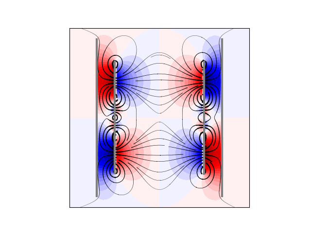
U = (U1 + U2).reshape(x.shape[0], y.shape[0])
U /= np.max(U)
plt.figure()
plt.contourf(X, Y, U.T, cmap="seismic", levels=40)
# plt.imshow(U, vmin=-1.0, vmax=1.0, cmap='seismic', interpolation='bicubic',
#           extent=(x.min(), x.max(), y.min(), y.max()))
plt.streamplot(
    x,
    y,
    B[1],
    B[0],
    density=2,
    linewidth=lw,
    color="k",
    start_points=seed_points.T,
    integration_direction="both",
    arrowsize=0.1,
)

# plt.plot(seed_points[0], seed_points[1], '*')

plt.plot(cx10, cy10, linewidth=3.0, color="gray")
plt.plot(cx20, cy20, linewidth=3.0, color="gray")
plt.plot(cx11, cy11, linewidth=3.0, color="gray")
plt.plot(cx21, cy21, linewidth=3.0, color="gray")
plt.axis("image")

plt.xticks([])
plt.yticks([])

Out:

([], <a list of 0 Text major ticklabel objects>)

N = 20
mm = max(abs(s1))
dd = 2 * mm / N
vmin = -dd * N / 2 + dd / 2
vmax = dd * N / 2 - dd / 2
contour_vals1 = np.arange(vmin, vmax, dd)
mm = max(abs(s2))
N2 = (2 * mm - dd) // dd
if N2 % 2 == 0:
    N2 -= 1
vmin = -dd * N2 / 2
vmax = mm
contour_vals2 = np.arange(vmin, vmax, dd)
contours1 = scalar_contour(mesh1, s1.vert, contours=contour_vals1)
contours2 = scalar_contour(mesh2, s2.vert, contours=contour_vals2)


def setscene(scene1, coil):
    scene1.actor.mapper.interpolate_scalars_before_mapping = True
    scene1.module_manager.scalar_lut_manager.number_of_colors = 32
    scene1.scene.y_plus_view()
    if coil == 1:
        scene1.scene.camera.position = [
            4.7267030067743576e-08,
            2.660205137153174,
            8.52196480605194e-08,
        ]
        scene1.scene.camera.focal_point = [
            4.7267030067743576e-08,
            0.4000000059604645,
            8.52196480605194e-08,
        ]
        scene1.scene.camera.view_angle = 30.0
        scene1.scene.camera.view_up = [1.0, 0.0, 0.0]
        scene1.scene.camera.clipping_range = [1.116284842928313, 2.4468228732691104]
        scene1.scene.camera.compute_view_plane_normal()
    else:
        scene1.scene.camera.position = [
            4.7267030067743576e-08,
            3.7091663385397116,
            8.52196480605194e-08,
        ]
        scene1.scene.camera.focal_point = [
            4.7267030067743576e-08,
            0.4000000059604645,
            8.52196480605194e-08,
        ]
        scene1.scene.camera.view_angle = 30.0
        scene1.scene.camera.view_up = [1.0, 0.0, 0.0]
        scene1.scene.camera.clipping_range = [2.948955346473114, 3.40878670176758]
        scene1.scene.camera.compute_view_plane_normal()
    scene1.scene.render()
    scene1.scene.anti_aliasing_frames = 20
    scene1.scene.magnification = 2


fig = mlab.figure(bgcolor=(1, 1, 1), size=(400, 400))
fig = plot_3d_current_loops(
    contours1, tube_radius=0.005, colors=(0.9, 0.9, 0.9), figure=fig
)
m = abs(s1).max()
mask = mesh1.triangles_center[:, 1] > 0
faces1 = mesh1.faces[mask]
surf = mlab.triangular_mesh(
    *mesh1.vertices.T, faces1, scalars=s1.vert, vmin=-m, vmax=m, colormap="seismic"
)
setscene(surf, 1)

fig = mlab.figure(bgcolor=(1, 1, 1), size=(400, 400))
fig = plot_3d_current_loops(
    contours2, tube_radius=0.005, colors=(0.9, 0.9, 0.9), figure=fig
)
faces2 = mesh2.faces[mesh2.triangles_center[:, 1] > 0]
surf = mlab.triangular_mesh(
    *mesh2.vertices.T, faces2, scalars=s2.vert, vmin=-m, vmax=m, colormap="seismic"
)
setscene(surf, 2)

• 
• 

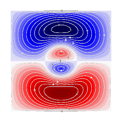
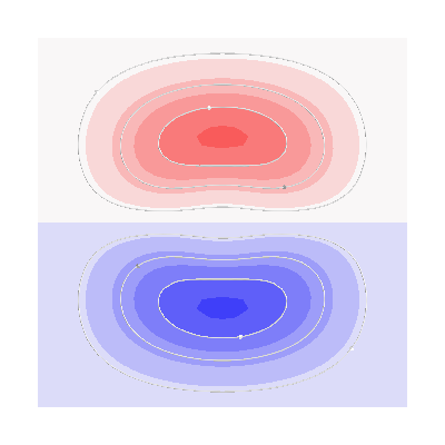
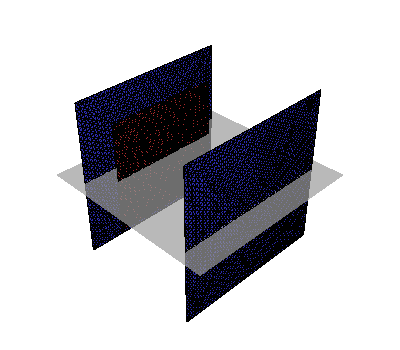
fig = mlab.figure(bgcolor=(1, 1, 1))
surf = mlab.triangular_mesh(*mesh1.vertices.T, mesh1.faces, color=(0.8, 0.2, 0.2))
surf.actor.property.edge_visibility = True
surf.actor.property.render_lines_as_tubes = True
surf.actor.property.line_width = 1.2


surf = mlab.triangular_mesh(*mesh2.vertices.T, mesh2.faces, color=(0.2, 0.2, 0.8))
surf.actor.property.edge_visibility = True
surf.actor.property.render_lines_as_tubes = True
surf.actor.property.line_width = 1.2
# Plot plane
plane = mlab.triangular_mesh(
    np.array([x[0], x[-1], x[-1], x[0]]),
    np.array([x[0], x[0], x[-1], x[-1]]),
    np.zeros(4),
    np.array([[0, 1, 2], [2, 3, 0]]),
    color=(0.7, 0.7, 0.7),
    opacity=0.7,
)

Estimated memory usage: 2077 MB